Methodology, Parameters, and Calculations
health economics methodology, clinical trial cost analysis, medical research ROI, cost-benefit analysis healthcare, sensitivity analysis, Monte Carlo simulation, DALY calculation, pragmatic clinical trials
Overview
This appendix documents all 55 parameters used in the analysis, organized by type:
- External sources (peer-reviewed): 27
- Calculated values: 23
- Core definitions: 5
Calculated Values
Parameters derived from mathematical formulas and economic models.
Annual Chronic Disease Patients Treated: 982M people
Estimated unique patients receiving chronic disease treatment annually. Derived from IQVIA days of therapy (1.28T) divided by 365 days divided by 2.5 average medications per patient times 70% post-1962 drugs.
Inputs:
- Annual Days of Chronic Disease Therapy 📊: 1.28T days (95% CI: 1.00T days - 1.50T days)
\[ \begin{gathered} N_{treated} \\ = DOT_{chronic} \times 0.000767 \\ = 1.28T \times 0.000767 \\ = 982M \end{gathered} \]
Methodology:57
? Low confidence
Sensitivity Analysis
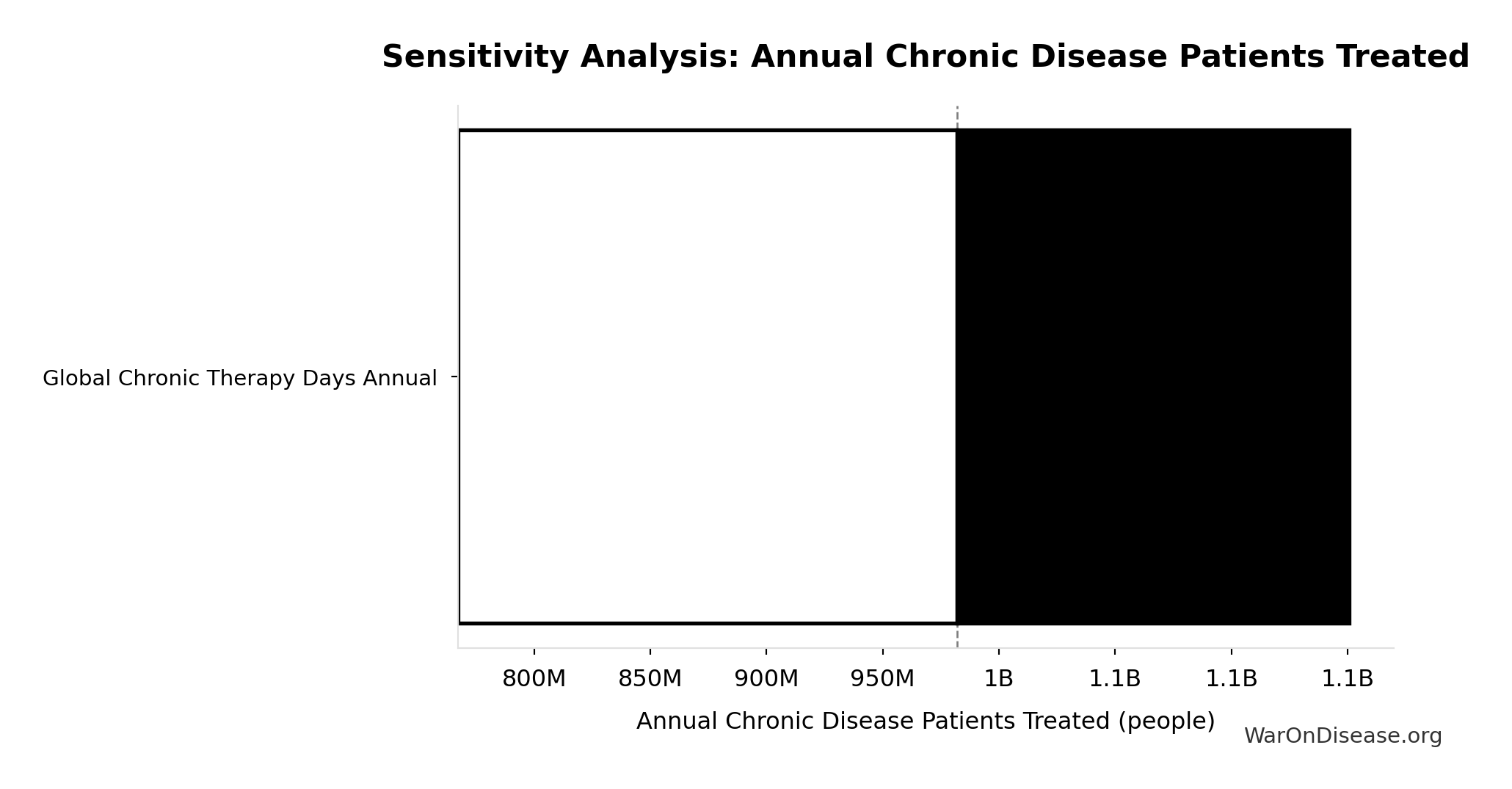
Sensitivity Indices for Annual Chronic Disease Patients Treated
Regression-based sensitivity showing which inputs explain the most variance in the output.
| Input Parameter | Sensitivity Coefficient | Interpretation |
|---|---|---|
| Global Chronic Therapy Days Annual | 1.0000 | Strong driver |
Interpretation: Standardized coefficients show the change in output (in SD units) per 1 SD change in input. Values near ±1 indicate strong influence; values exceeding ±1 may occur with correlated inputs.
Monte Carlo Distribution
Simulation Results Summary: Annual Chronic Disease Patients Treated
| Statistic | Value |
|---|---|
| Baseline (deterministic) | 982M |
| Mean (expected value) | 981M |
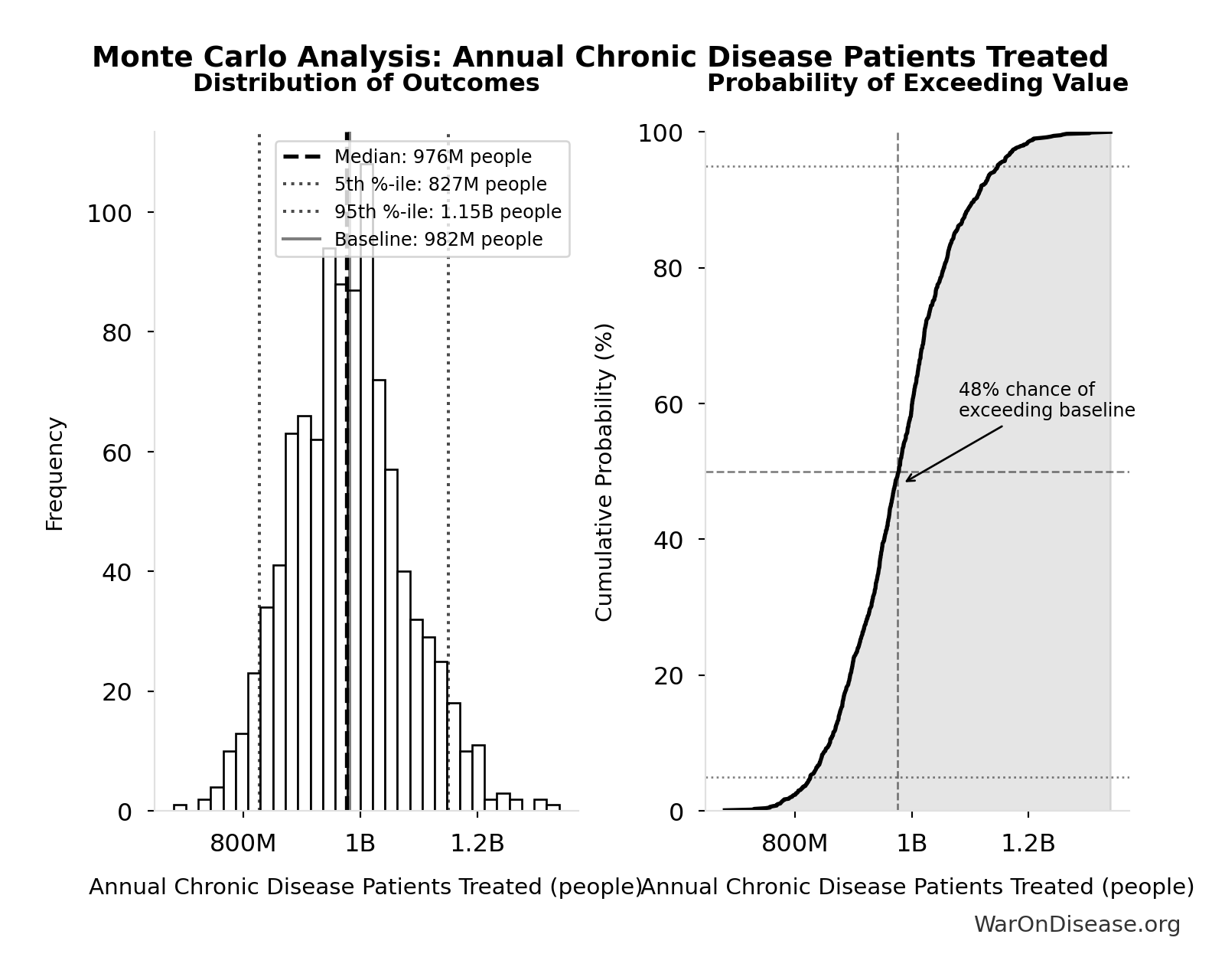
| Median (50th percentile) | 976M |
| Standard Deviation | 98.4M |
| 90% Confidence Interval | [827M, 1.15B] |
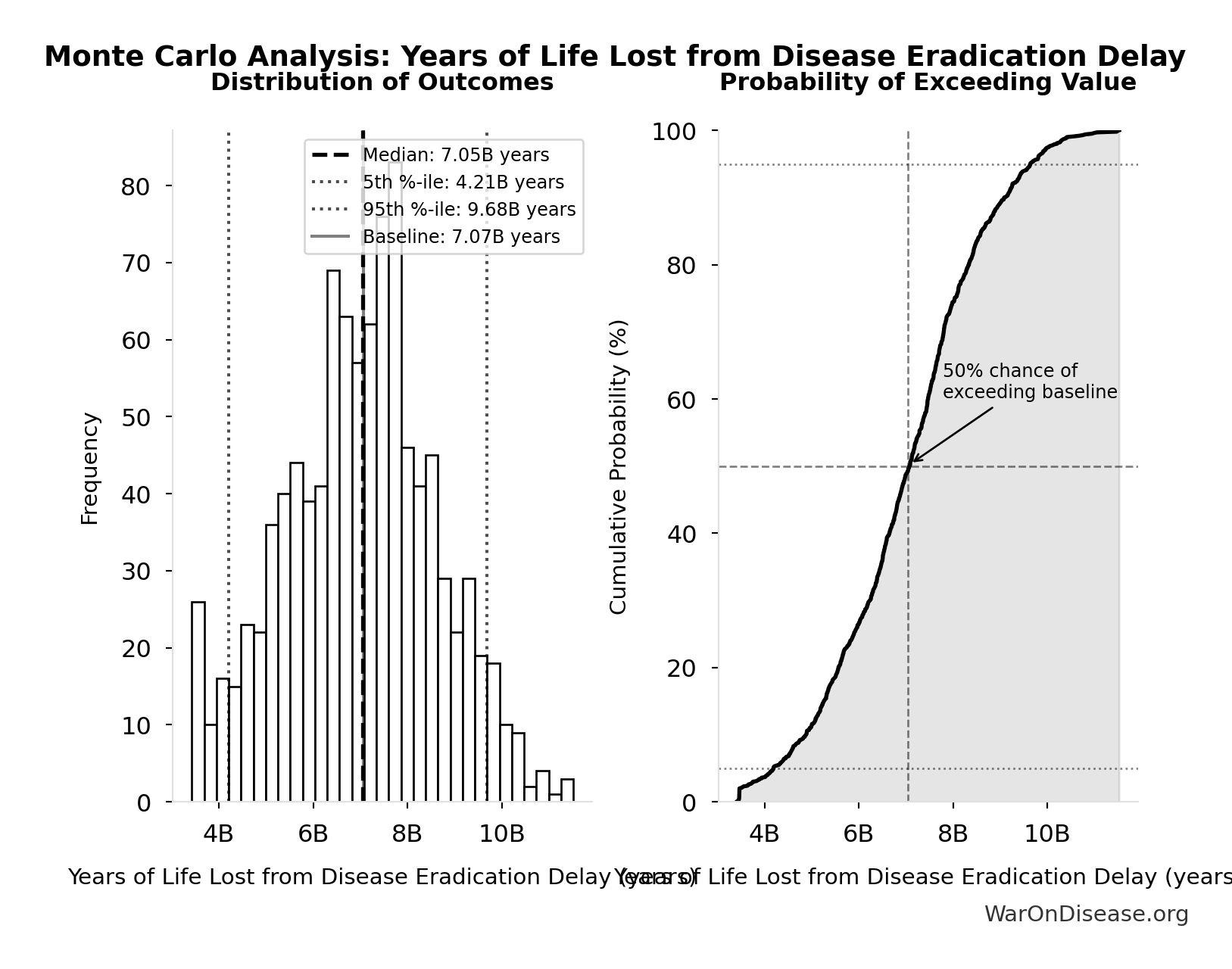
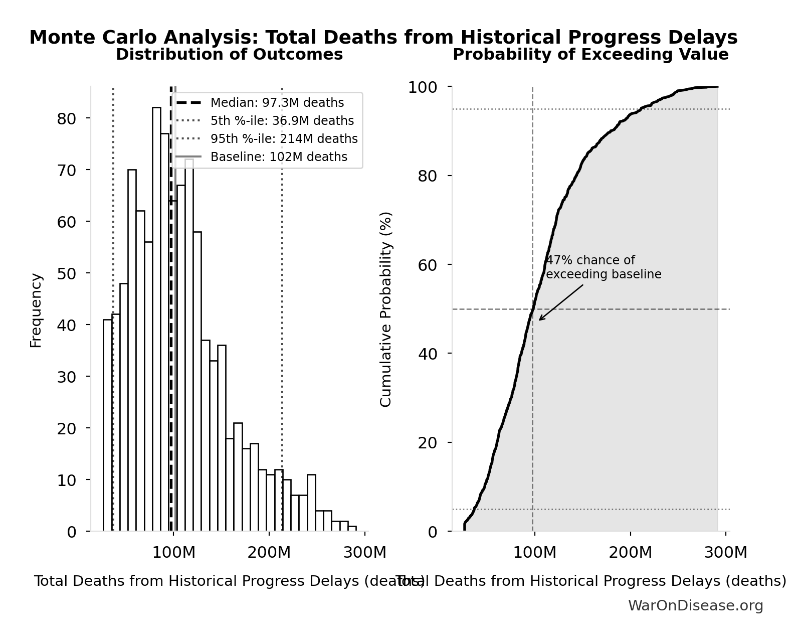
The histogram shows the distribution of Annual Chronic Disease Patients Treated across 10,000 Monte Carlo simulations. The CDF (right) shows the probability of the outcome exceeding any given value, which is useful for risk assessment.
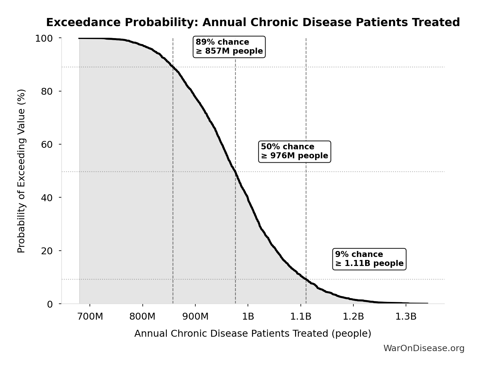
Exceedance Probability
This exceedance probability chart shows the likelihood that Annual Chronic Disease Patients Treated will exceed any given threshold. Higher curves indicate more favorable outcomes with greater certainty.
Total DALYs Lost from Disease Eradication Delay: 7.94B DALYs
Total Disability-Adjusted Life Years lost from disease eradication delay (PRIMARY estimate)
Inputs:
- Years of Life Lost from Disease Eradication Delay 🔢: 7.07B years
- Years Lived with Disability During Disease Eradication Delay 🔢: 873M years
\[ \begin{gathered} DALYs_{lag} = YLL_{lag} + YLD_{lag} = 7.07B + 873M = 7.94B \\[0.5em] \text{where } YLL_{lag} \\ = Deaths_{lag} \times (LE_{global} - Age_{death,delay}) \\ = 416M \times (79 - 62) \\ = 7.07B \\[0.5em] \text{where } Deaths_{lag} \\ = T_{lag} \times Deaths_{disease,daily} \times 338 \\ = 8.2 \times 150{,}000 \times 338 \\ = 416M \\[0.5em] \text{where } YLD_{lag} \\ = Deaths_{lag} \times T_{suffering} \times DW_{chronic} \\ = 416M \times 6 \times 0.35 \\ = 873M \\[0.5em] \text{where } Deaths_{lag} \\ = T_{lag} \times Deaths_{disease,daily} \times 338 \\ = 8.2 \times 150{,}000 \times 338 \\ = 416M \end{gathered} \]
Methodology: ../appendix/invisible-graveyard#daly-calculation
~ Medium confidence
Sensitivity Analysis
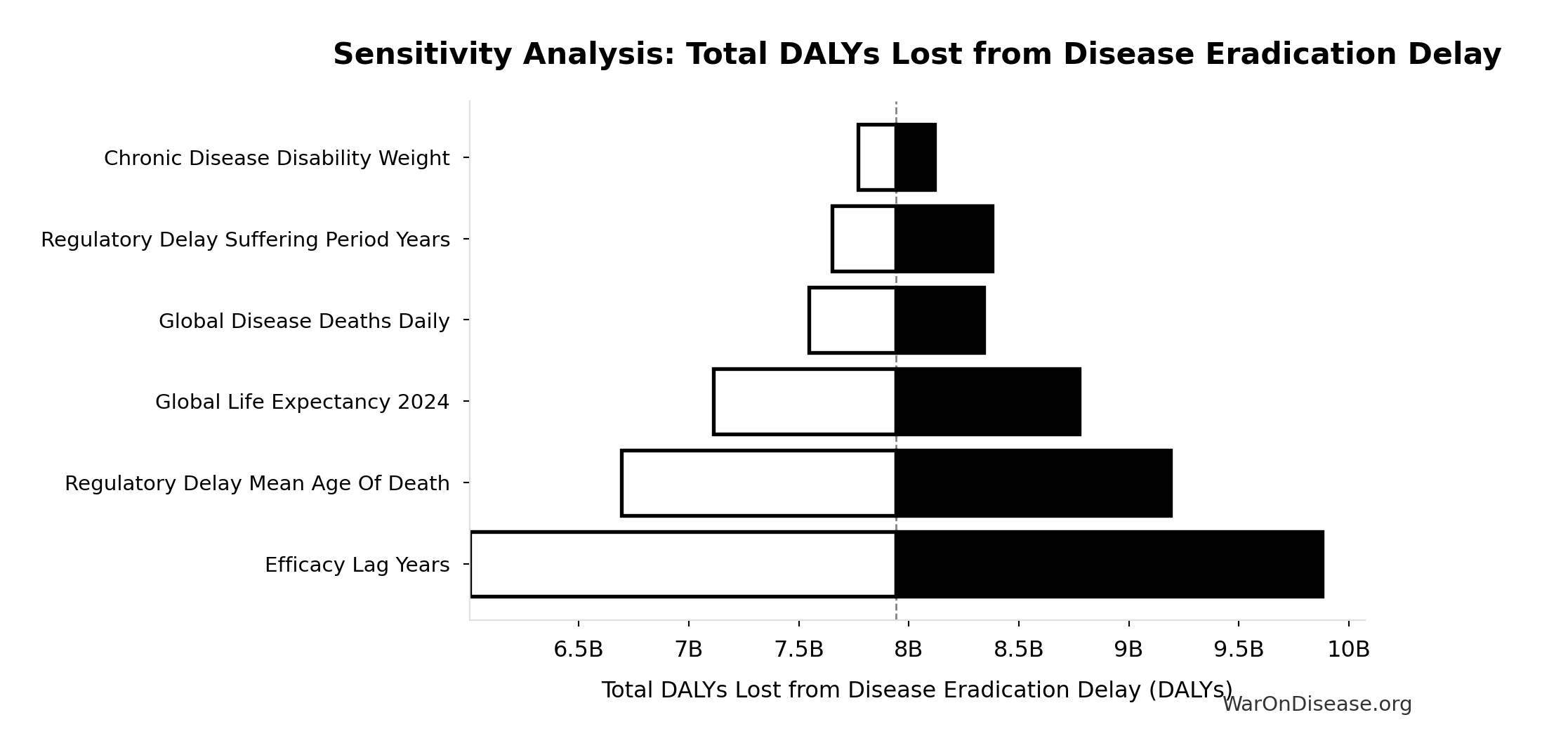
Sensitivity Indices for Total DALYs Lost from Disease Eradication Delay
Regression-based sensitivity showing which inputs explain the most variance in the output.
| Input Parameter | Sensitivity Coefficient | Interpretation |
|---|---|---|
| dFDA Efficacy Lag Elimination Yll | 0.7043 | Strong driver |
| dFDA Efficacy Lag Elimination Yld | 0.3107 | Moderate driver |
Interpretation: Standardized coefficients show the change in output (in SD units) per 1 SD change in input. Values near ±1 indicate strong influence; values exceeding ±1 may occur with correlated inputs.
Monte Carlo Distribution
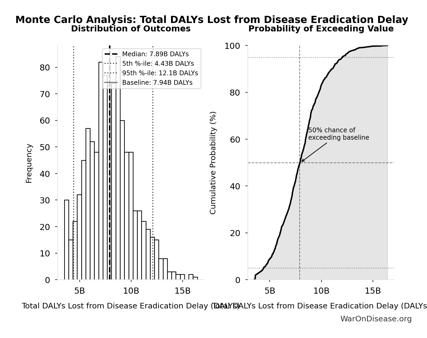
Simulation Results Summary: Total DALYs Lost from Disease Eradication Delay
| Statistic | Value |
|---|---|
| Baseline (deterministic) | 7.94B |
| Mean (expected value) | 8.05B |
| Median (50th percentile) | 7.89B |
| Standard Deviation | 2.31B |
| 90% Confidence Interval | [4.43B, 12.1B] |
The histogram shows the distribution of Total DALYs Lost from Disease Eradication Delay across 10,000 Monte Carlo simulations. The CDF (right) shows the probability of the outcome exceeding any given value, which is useful for risk assessment.
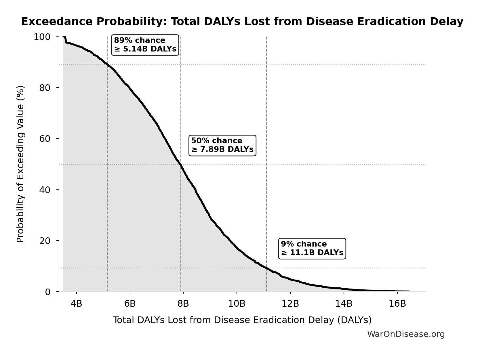
Exceedance Probability
This exceedance probability chart shows the likelihood that Total DALYs Lost from Disease Eradication Delay will exceed any given threshold. Higher curves indicate more favorable outcomes with greater certainty.
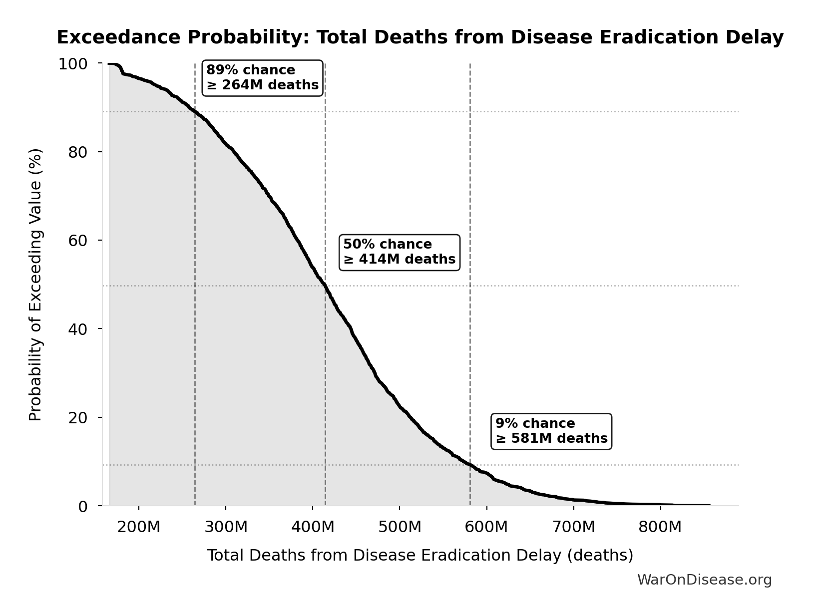
Total Deaths from Disease Eradication Delay: 416M deaths
Total eventually avoidable deaths from delaying disease eradication by 8.2 years (PRIMARY estimate, conservative). Excludes fundamentally unavoidable deaths (primarily accidents ~7.9%).
Inputs:
- Regulatory Delay for Efficacy Testing Post-Safety Verification 📊: 8.2 years (SE: ±2 years)
- Global Daily Deaths from Disease and Aging 📊: 150k deaths/day (SE: ±7.50k deaths/day)
\[ \begin{gathered} Deaths_{lag} \\ = T_{lag} \times Deaths_{disease,daily} \times 338 \\ = 8.2 \times 150{,}000 \times 338 \\ = 416M \end{gathered} \]
Methodology: ../appendix/invisible-graveyard#disease-eradication-delay
~ Medium confidence
Sensitivity Analysis
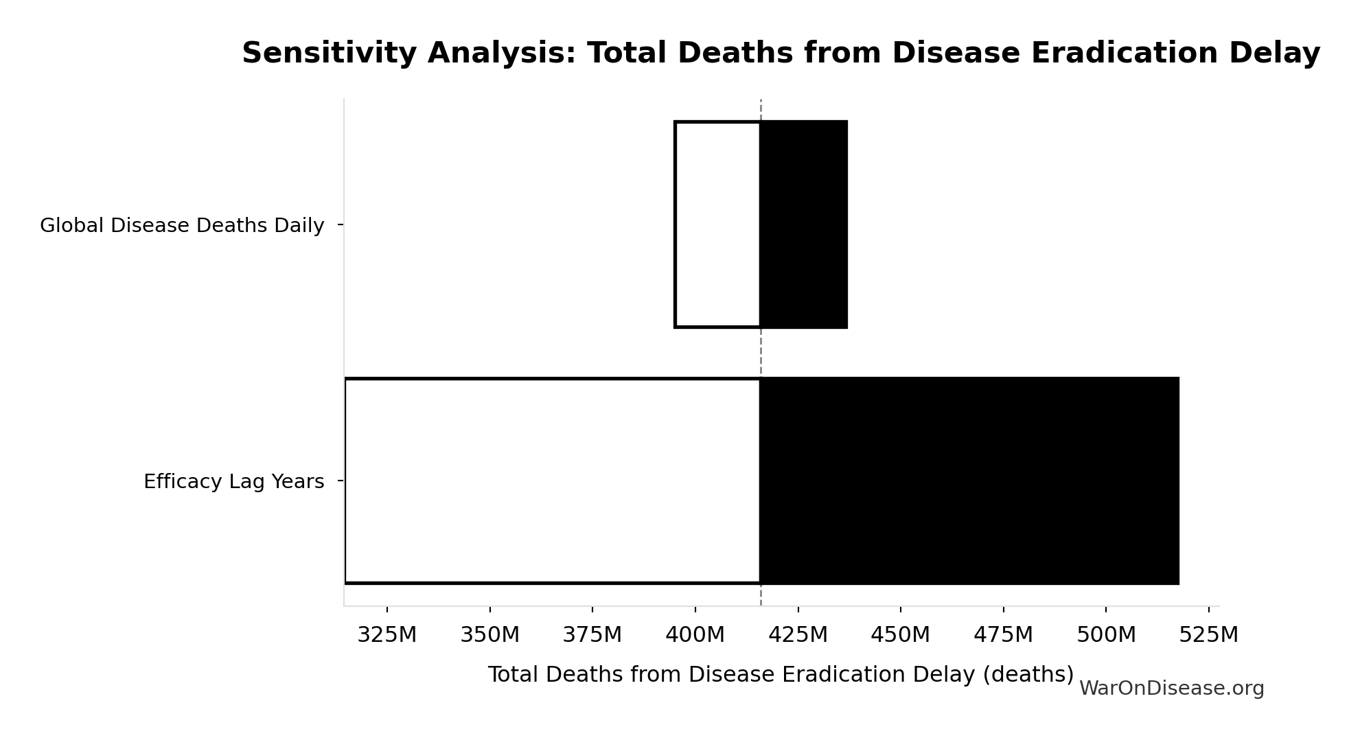
Sensitivity Indices for Total Deaths from Disease Eradication Delay
Regression-based sensitivity showing which inputs explain the most variance in the output.
| Input Parameter | Sensitivity Coefficient | Interpretation |
|---|---|---|
| Efficacy Lag Years | 1.1404 | Strong driver |
| Global Disease Deaths Daily | -0.1422 | Weak driver |
Interpretation: Standardized coefficients show the change in output (in SD units) per 1 SD change in input. Values near ±1 indicate strong influence; values exceeding ±1 may occur with correlated inputs.
Monte Carlo Distribution
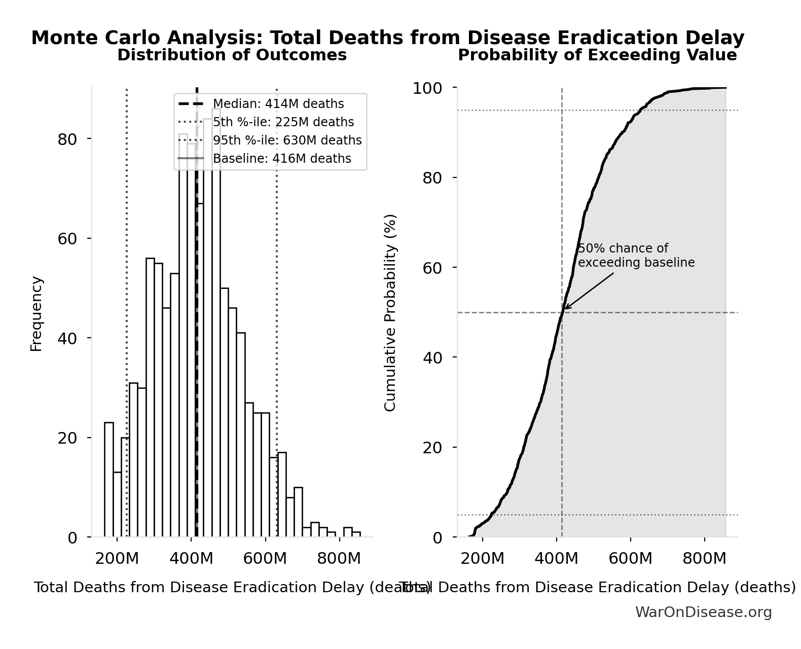
Simulation Results Summary: Total Deaths from Disease Eradication Delay
| Statistic | Value |
|---|---|
| Baseline (deterministic) | 416M |
| Mean (expected value) | 420M |
| Median (50th percentile) | 414M |
| Standard Deviation | 122M |
| 90% Confidence Interval | [225M, 630M] |
The histogram shows the distribution of Total Deaths from Disease Eradication Delay across 10,000 Monte Carlo simulations. The CDF (right) shows the probability of the outcome exceeding any given value, which is useful for risk assessment.
Exceedance Probability
This exceedance probability chart shows the likelihood that Total Deaths from Disease Eradication Delay will exceed any given threshold. Higher curves indicate more favorable outcomes with greater certainty.
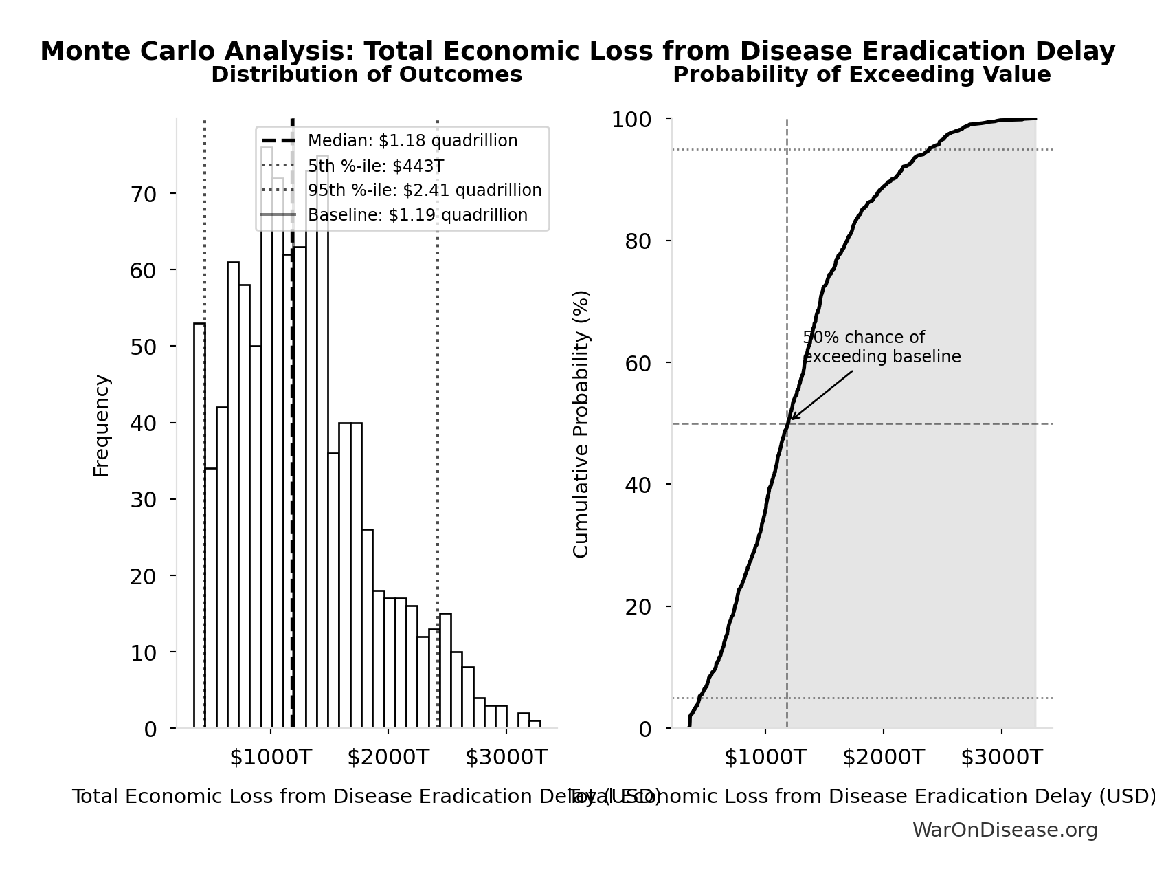
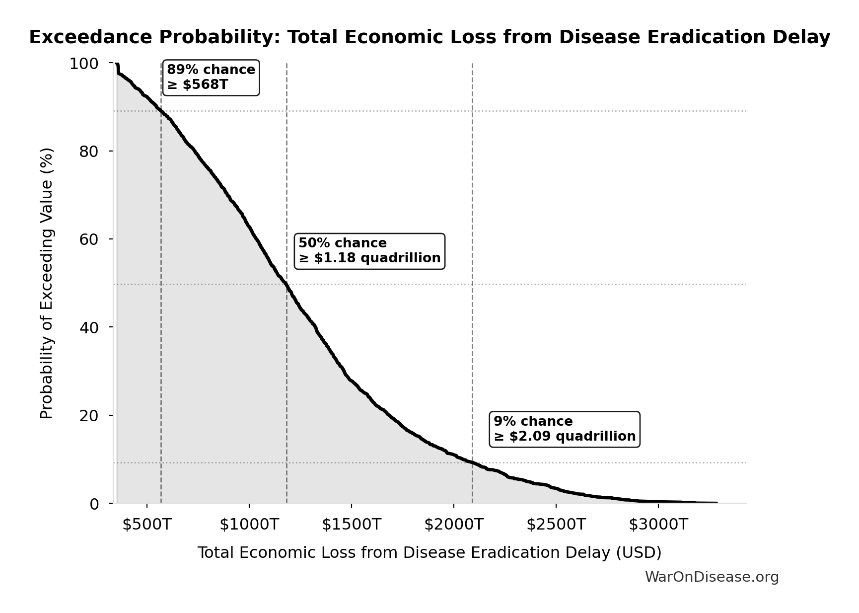
Total Economic Loss from Disease Eradication Delay: $1.19 quadrillion
Total economic loss from delaying disease eradication by 8.2 years (PRIMARY estimate, 2024 USD). Values global DALYs at standardized US/International normative rate ($150k) rather than local ability-to-pay, representing the full human capital loss.
Inputs:
- Total DALYs Lost from Disease Eradication Delay 🔢: 7.94B DALYs
- Standard Economic Value per QALY 📊: $150K (SE: ±$30K)
\[ \begin{gathered} Value_{lag} \\ = DALYs_{lag} \times Value_{QALY} \\ = 7.94B \times \$150K \\ = \$1190T \\[0.5em] \text{where } DALYs_{lag} = YLL_{lag} + YLD_{lag} = 7.07B + 873M = 7.94B \\[0.5em] \text{where } YLL_{lag} \\ = Deaths_{lag} \times (LE_{global} - Age_{death,delay}) \\ = 416M \times (79 - 62) \\ = 7.07B \\[0.5em] \text{where } Deaths_{lag} \\ = T_{lag} \times Deaths_{disease,daily} \times 338 \\ = 8.2 \times 150{,}000 \times 338 \\ = 416M \\[0.5em] \text{where } YLD_{lag} \\ = Deaths_{lag} \times T_{suffering} \times DW_{chronic} \\ = 416M \times 6 \times 0.35 \\ = 873M \\[0.5em] \text{where } Deaths_{lag} \\ = T_{lag} \times Deaths_{disease,daily} \times 338 \\ = 8.2 \times 150{,}000 \times 338 \\ = 416M \end{gathered} \]
Methodology: ../appendix/invisible-graveyard#economic-valuation
~ Medium confidence
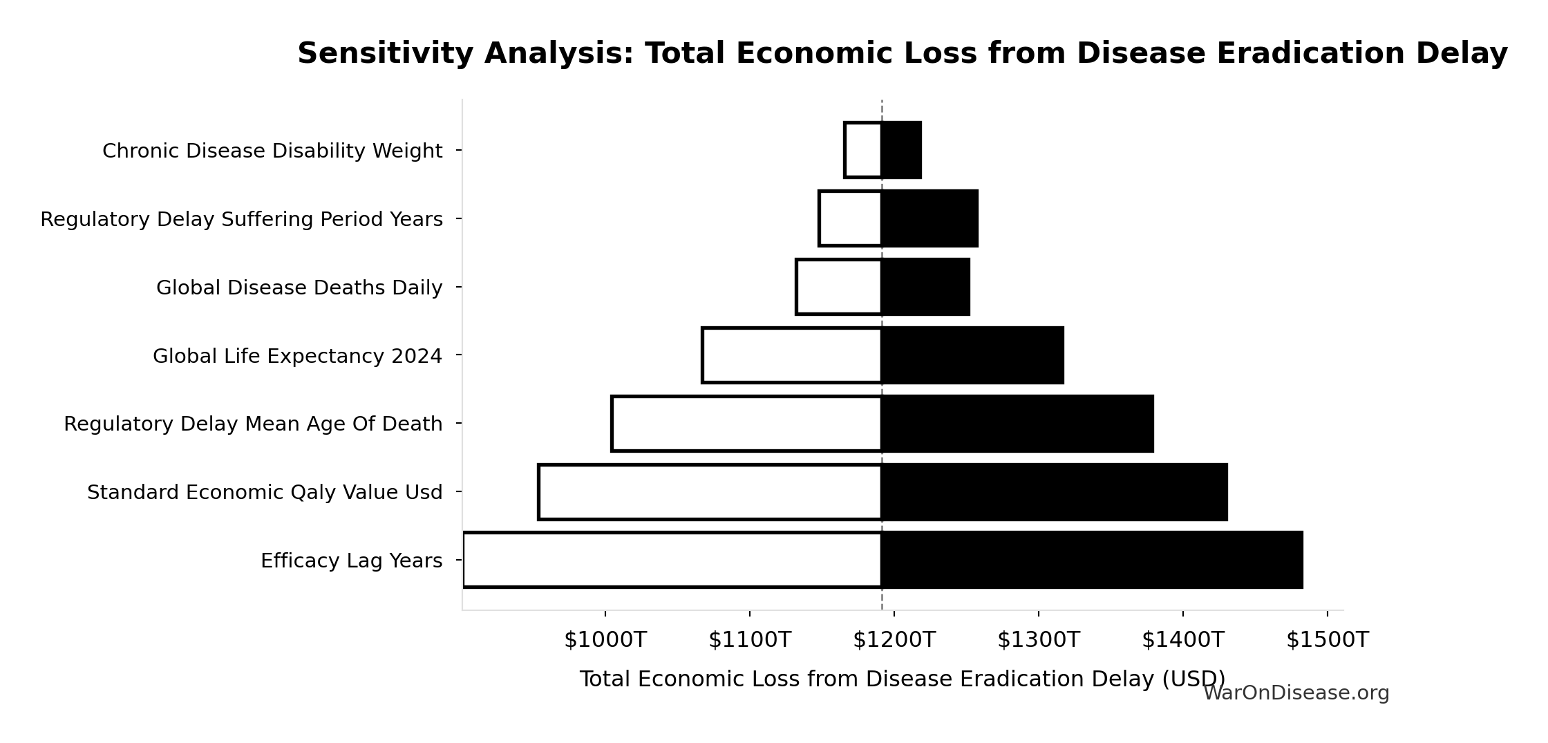
Sensitivity Analysis
Sensitivity Indices for Total Economic Loss from Disease Eradication Delay
Regression-based sensitivity showing which inputs explain the most variance in the output.
| Input Parameter | Sensitivity Coefficient | Interpretation |
|---|---|---|
| dFDA Efficacy Lag Elimination DALYs | 1.0671 | Strong driver |
| Standard Economic QALY Value Usd | -0.0733 | Minimal effect |
Interpretation: Standardized coefficients show the change in output (in SD units) per 1 SD change in input. Values near ±1 indicate strong influence; values exceeding ±1 may occur with correlated inputs.
Monte Carlo Distribution
Simulation Results Summary: Total Economic Loss from Disease Eradication Delay
| Statistic | Value |
|---|---|
| Baseline (deterministic) | $1.19 quadrillion |
| Mean (expected value) | $1.27 quadrillion |
| Median (50th percentile) | $1.18 quadrillion |
| Standard Deviation | $581T |
| 90% Confidence Interval | [$443T, $2.41 quadrillion] |
The histogram shows the distribution of Total Economic Loss from Disease Eradication Delay across 10,000 Monte Carlo simulations. The CDF (right) shows the probability of the outcome exceeding any given value, which is useful for risk assessment.
Exceedance Probability
This exceedance probability chart shows the likelihood that Total Economic Loss from Disease Eradication Delay will exceed any given threshold. Higher curves indicate more favorable outcomes with greater certainty.
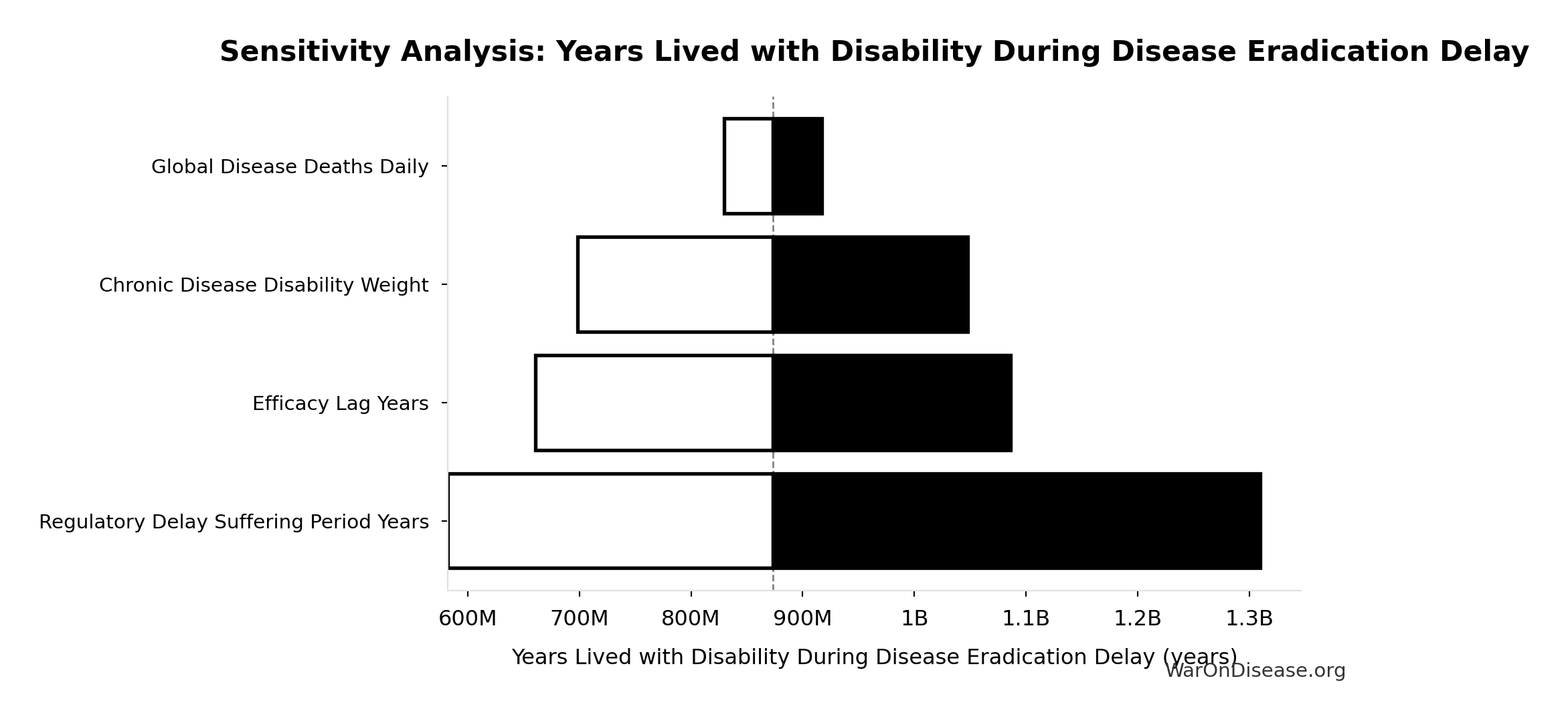
Years Lived with Disability During Disease Eradication Delay: 873M years
Years Lived with Disability during disease eradication delay (PRIMARY estimate)
Inputs:
- Total Deaths from Disease Eradication Delay 🔢: 416M deaths
- Pre-Death Suffering Period During Post-Safety Efficacy Delay 📊: 6 years (95% CI: 4 years - 9 years)
- Disability Weight for Untreated Chronic Conditions 📊: 0.35 weight (SE: ±0.07 weight)
\[ \begin{gathered} YLD_{lag} \\ = Deaths_{lag} \times T_{suffering} \times DW_{chronic} \\ = 416M \times 6 \times 0.35 \\ = 873M \\[0.5em] \text{where } Deaths_{lag} \\ = T_{lag} \times Deaths_{disease,daily} \times 338 \\ = 8.2 \times 150{,}000 \times 338 \\ = 416M \end{gathered} \]
Methodology: ../appendix/invisible-graveyard#daly-calculation
~ Medium confidence
Sensitivity Analysis
Sensitivity Indices for Years Lived with Disability During Disease Eradication Delay
Regression-based sensitivity showing which inputs explain the most variance in the output.
| Input Parameter | Sensitivity Coefficient | Interpretation |
|---|---|---|
| Regulatory Delay Suffering Period Years | 2.0883 | Strong driver |
| Chronic Disease Disability Weight | -0.9003 | Strong driver |
| dFDA Efficacy Lag Elimination Deaths Averted | -0.2255 | Weak driver |
Interpretation: Standardized coefficients show the change in output (in SD units) per 1 SD change in input. Values near ±1 indicate strong influence; values exceeding ±1 may occur with correlated inputs.
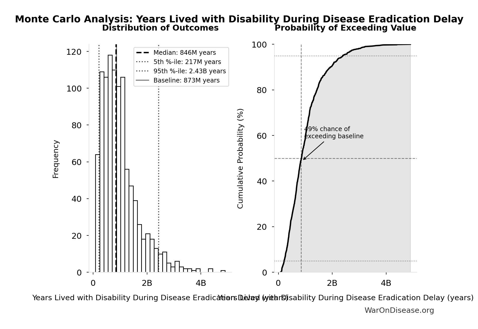
Monte Carlo Distribution
Simulation Results Summary: Years Lived with Disability During Disease Eradication Delay
| Statistic | Value |
|---|---|
| Baseline (deterministic) | 873M |
| Mean (expected value) | 1.02B |
| Median (50th percentile) | 846M |
| Standard Deviation | 716M |
| 90% Confidence Interval | [217M, 2.43B] |
The histogram shows the distribution of Years Lived with Disability During Disease Eradication Delay across 10,000 Monte Carlo simulations. The CDF (right) shows the probability of the outcome exceeding any given value, which is useful for risk assessment.
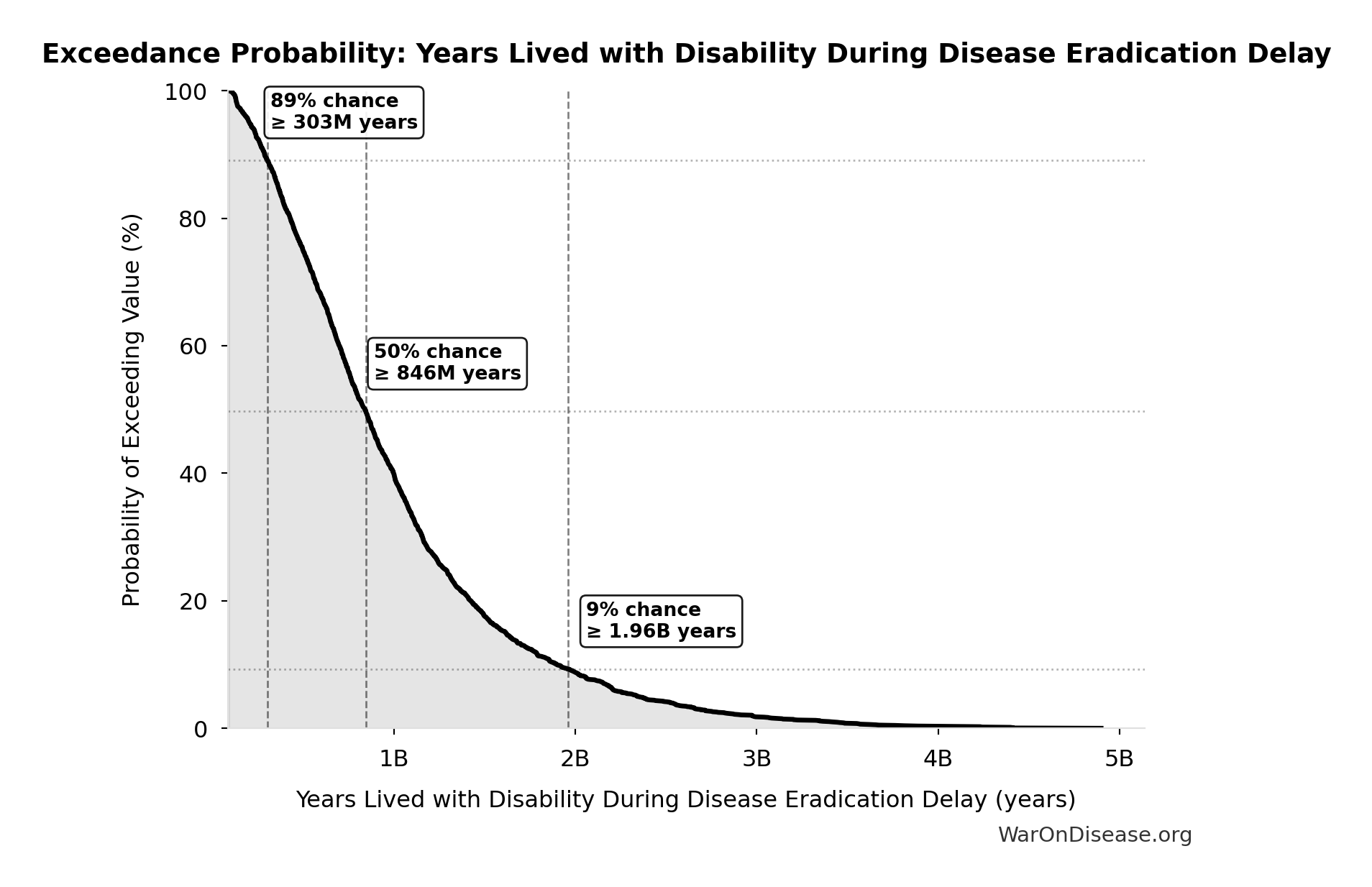
Exceedance Probability
This exceedance probability chart shows the likelihood that Years Lived with Disability During Disease Eradication Delay will exceed any given threshold. Higher curves indicate more favorable outcomes with greater certainty.
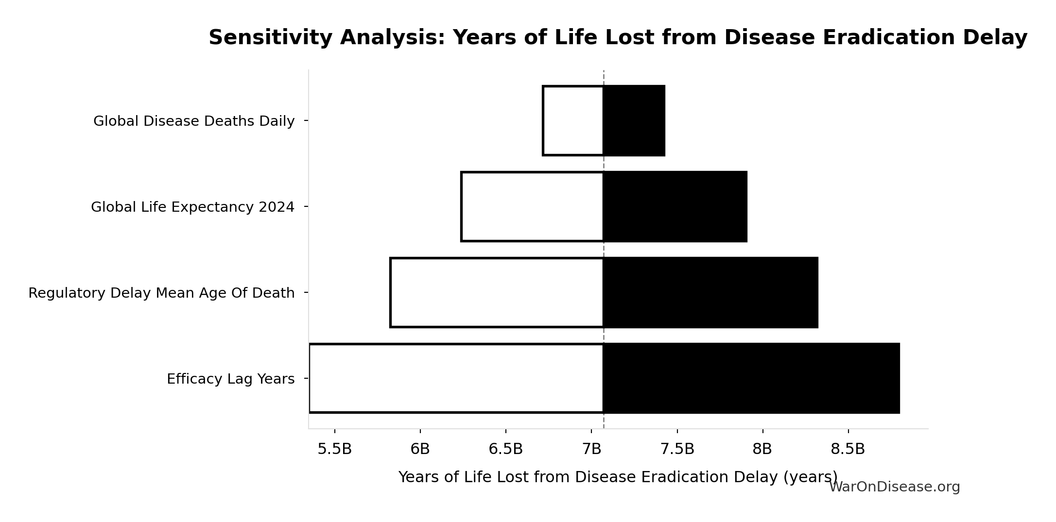
Years of Life Lost from Disease Eradication Delay: 7.07B years
Years of Life Lost from disease eradication delay deaths (PRIMARY estimate)
Inputs:
- Total Deaths from Disease Eradication Delay 🔢: 416M deaths
- Global Life Expectancy (2024) 📊: 79 years (SE: ±2 years)
- Mean Age of Preventable Death from Post-Safety Efficacy Delay 📊: 62 years (SE: ±3 years)
\[ \begin{gathered} YLL_{lag} \\ = Deaths_{lag} \times (LE_{global} - Age_{death,delay}) \\ = 416M \times (79 - 62) \\ = 7.07B \\[0.5em] \text{where } Deaths_{lag} \\ = T_{lag} \times Deaths_{disease,daily} \times 338 \\ = 8.2 \times 150{,}000 \times 338 \\ = 416M \end{gathered} \]
Methodology: ../appendix/invisible-graveyard#daly-calculation
~ Medium confidence
Sensitivity Analysis
Sensitivity Indices for Years of Life Lost from Disease Eradication Delay
Regression-based sensitivity showing which inputs explain the most variance in the output.
| Input Parameter | Sensitivity Coefficient | Interpretation |
|---|---|---|
| Global Life Expectancy 2024 | 2.0066 | Strong driver |
| Regulatory Delay Mean Age Of Death | -1.3852 | Strong driver |
| dFDA Efficacy Lag Elimination Deaths Averted | 0.3779 | Moderate driver |
Interpretation: Standardized coefficients show the change in output (in SD units) per 1 SD change in input. Values near ±1 indicate strong influence; values exceeding ±1 may occur with correlated inputs.
Monte Carlo Distribution
Simulation Results Summary: Years of Life Lost from Disease Eradication Delay
| Statistic | Value |
|---|---|
| Baseline (deterministic) | 7.07B |
| Mean (expected value) | 7.03B |
| Median (50th percentile) | 7.05B |
| Standard Deviation | 1.62B |
| 90% Confidence Interval | [4.21B, 9.68B] |
The histogram shows the distribution of Years of Life Lost from Disease Eradication Delay across 10,000 Monte Carlo simulations. The CDF (right) shows the probability of the outcome exceeding any given value, which is useful for risk assessment.
Exceedance Probability
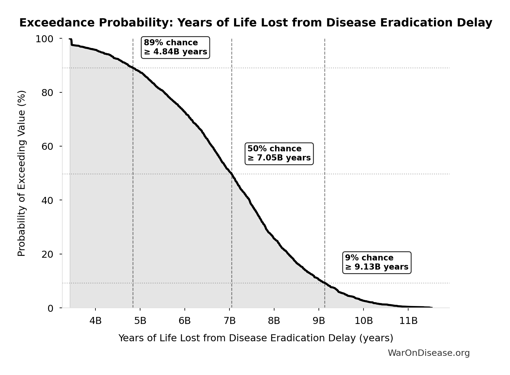
This exceedance probability chart shows the likelihood that Years of Life Lost from Disease Eradication Delay will exceed any given threshold. Higher curves indicate more favorable outcomes with greater certainty.
dFDA Trial Cost Reduction Percentage: 97.7%
Trial cost reduction percentage: (traditional - dFDA) / traditional = ($41K - $1.2K) / $41K = 97%
Inputs:
- dFDA Pragmatic Trial Cost per Patient 📊: $929 (95% CI: $97 - $3K)
- Phase 3 Cost per Patient 📊: $41K (95% CI: $20K - $120K)
\[ \begin{gathered} Reduce_{pct} \\ = 1 - \frac{Cost_{pragmatic,pt}}{Cost_{P3,pt}} \\ = 1 - \frac{\$929}{\$41K} \\ = 97.7\% \end{gathered} \]
Methodology: ../appendix/dfda-impact-paper#cost-reduction
✓ High confidence
Sensitivity Analysis
Sensitivity Indices for dFDA Trial Cost Reduction Percentage
Regression-based sensitivity showing which inputs explain the most variance in the output.
| Input Parameter | Sensitivity Coefficient | Interpretation |
|---|---|---|
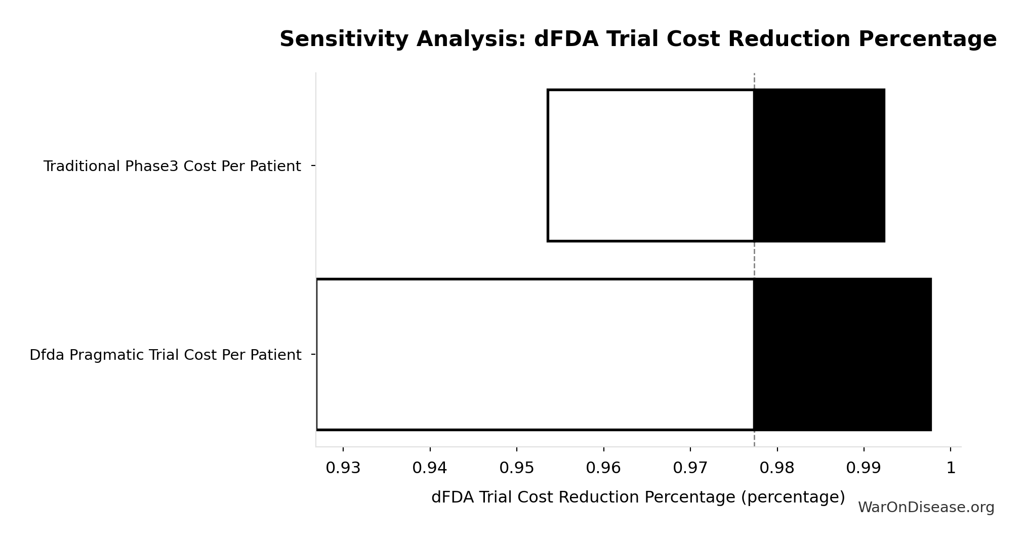
| dFDA Pragmatic Trial Cost Per Patient | -6.4207 | Strong driver |
| Traditional Phase3 Cost Per Patient | 5.6539 | Strong driver |
Interpretation: Standardized coefficients show the change in output (in SD units) per 1 SD change in input. Values near ±1 indicate strong influence; values exceeding ±1 may occur with correlated inputs.
Monte Carlo Distribution
Simulation Results Summary: dFDA Trial Cost Reduction Percentage
| Statistic | Value |
|---|---|
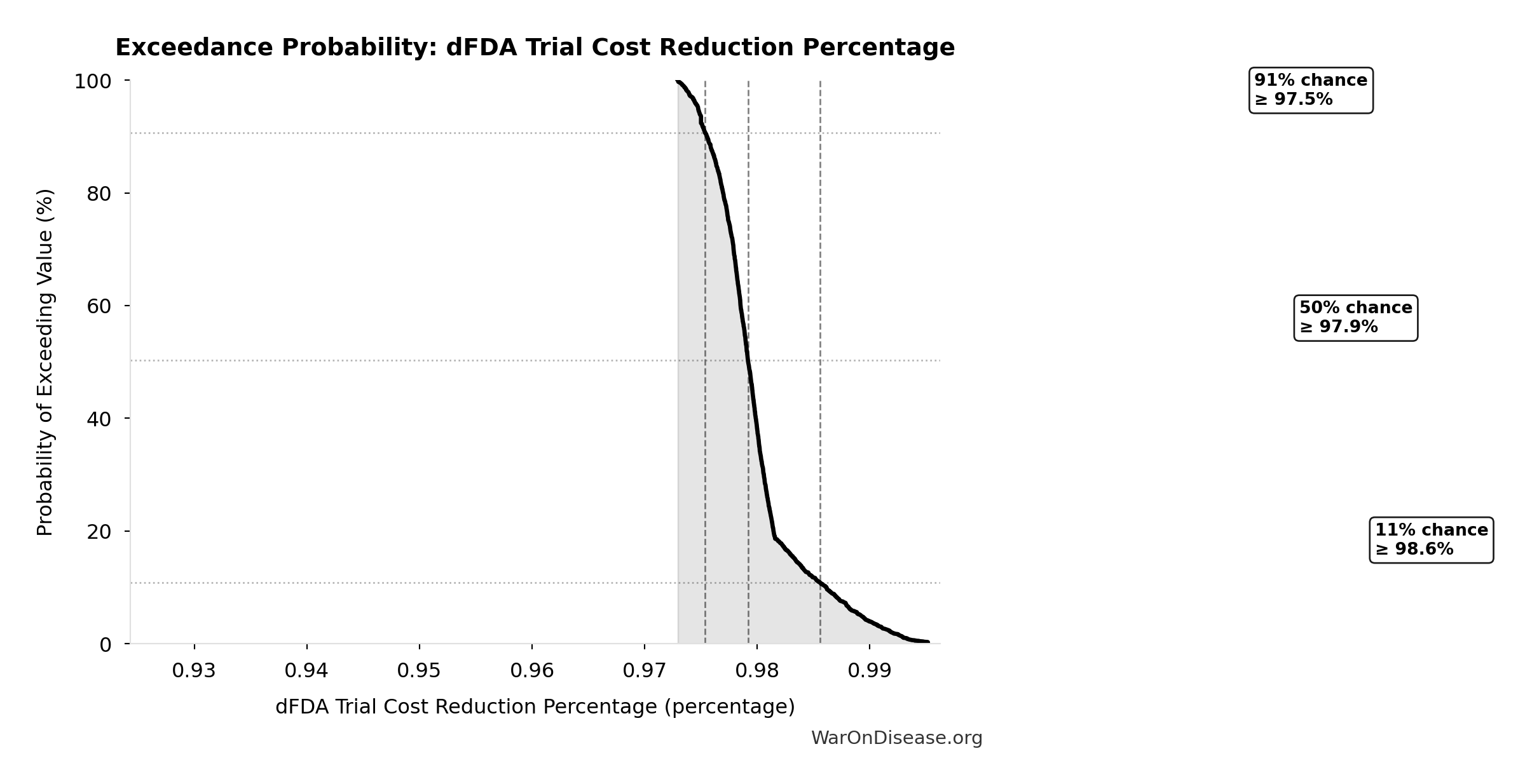
| Baseline (deterministic) | 97.7% |
| Mean (expected value) | 98% |
| Median (50th percentile) | 97.9% |
| Standard Deviation | 0.401% |
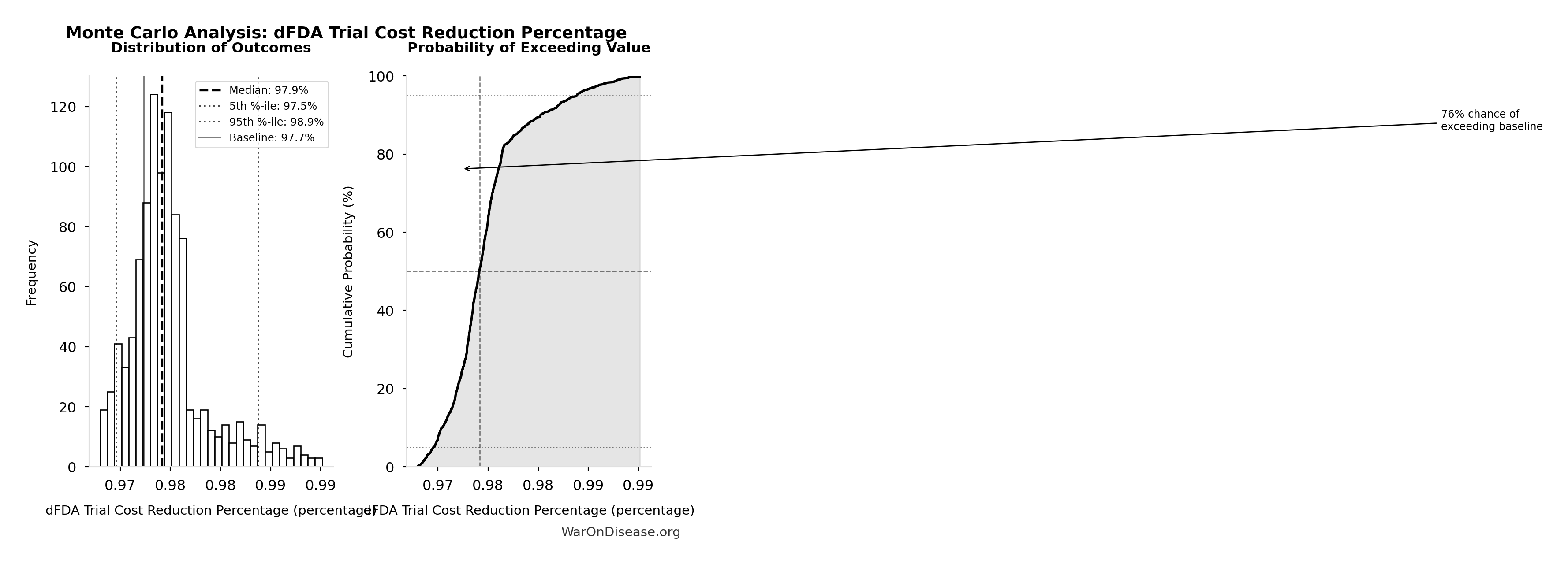
| 90% Confidence Interval | [97.5%, 98.9%] |
The histogram shows the distribution of dFDA Trial Cost Reduction Percentage across 10,000 Monte Carlo simulations. The CDF (right) shows the probability of the outcome exceeding any given value, which is useful for risk assessment.
Exceedance Probability
This exceedance probability chart shows the likelihood that dFDA Trial Cost Reduction Percentage will exceed any given threshold. Higher curves indicate more favorable outcomes with greater certainty.
Diseases Without Effective Treatment: 6.65k diseases
Number of diseases without effective treatment. 95% of 7,000 rare diseases lack FDA-approved treatment (per Orphanet 2024). This is the ‘queue’ of diseases waiting for cures.
Inputs:
- Total Number of Rare Diseases Globally 📊: 7.00k diseases (95% CI: 6.00k diseases - 10.0k diseases)
\[ \begin{gathered} N_{untreated} \\ = N_{rare} \times 0.95 \\ = 7{,}000 \times 0.95 \\ = 6{,}650 \end{gathered} \]
Methodology:142
~ Medium confidence
Sensitivity Analysis
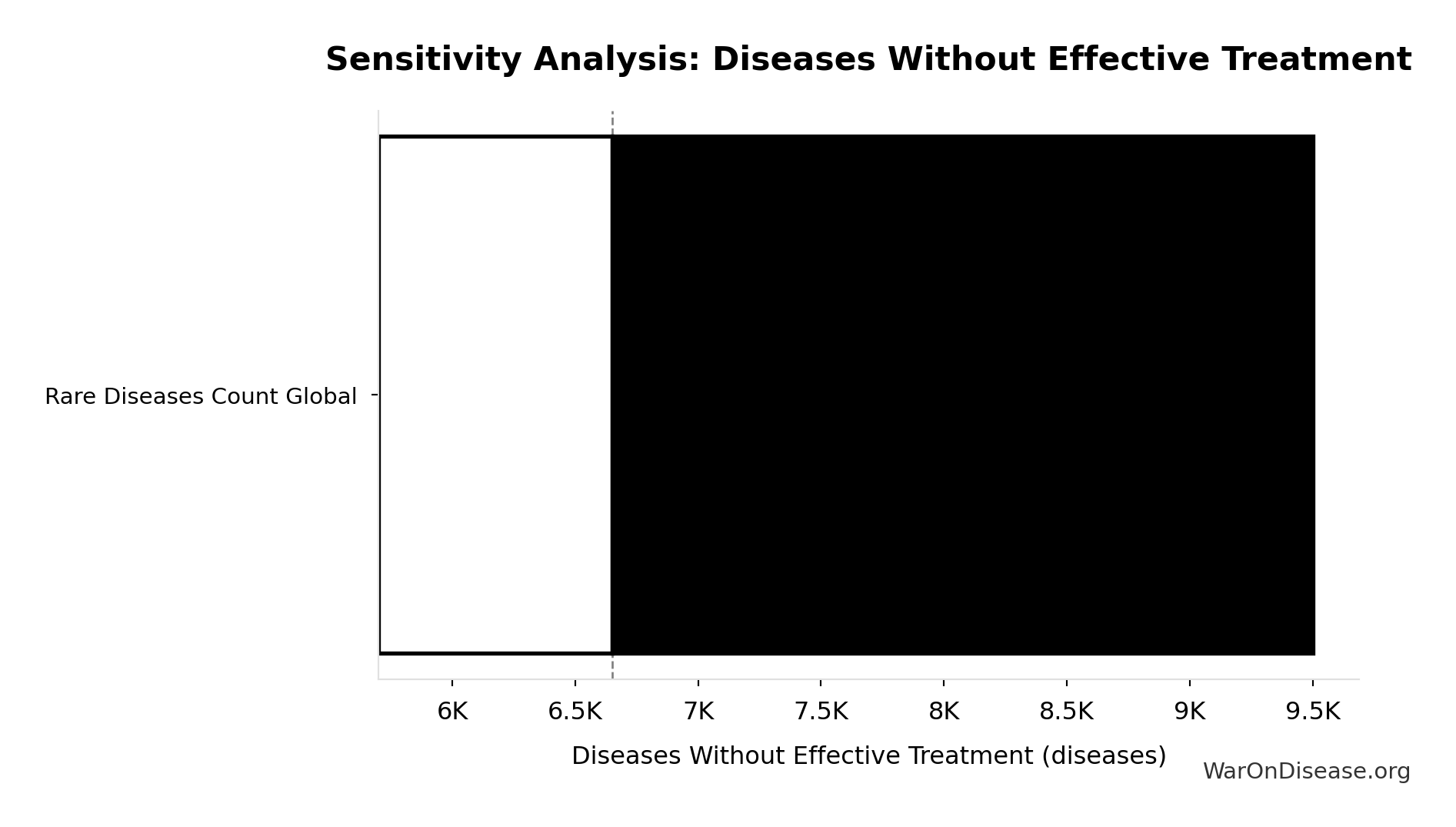
Sensitivity Indices for Diseases Without Effective Treatment
Regression-based sensitivity showing which inputs explain the most variance in the output.
| Input Parameter | Sensitivity Coefficient | Interpretation |
|---|---|---|
| Rare Diseases Count Global | 1.0000 | Strong driver |
Interpretation: Standardized coefficients show the change in output (in SD units) per 1 SD change in input. Values near ±1 indicate strong influence; values exceeding ±1 may occur with correlated inputs.
Monte Carlo Distribution
Simulation Results Summary: Diseases Without Effective Treatment
| Statistic | Value |
|---|---|
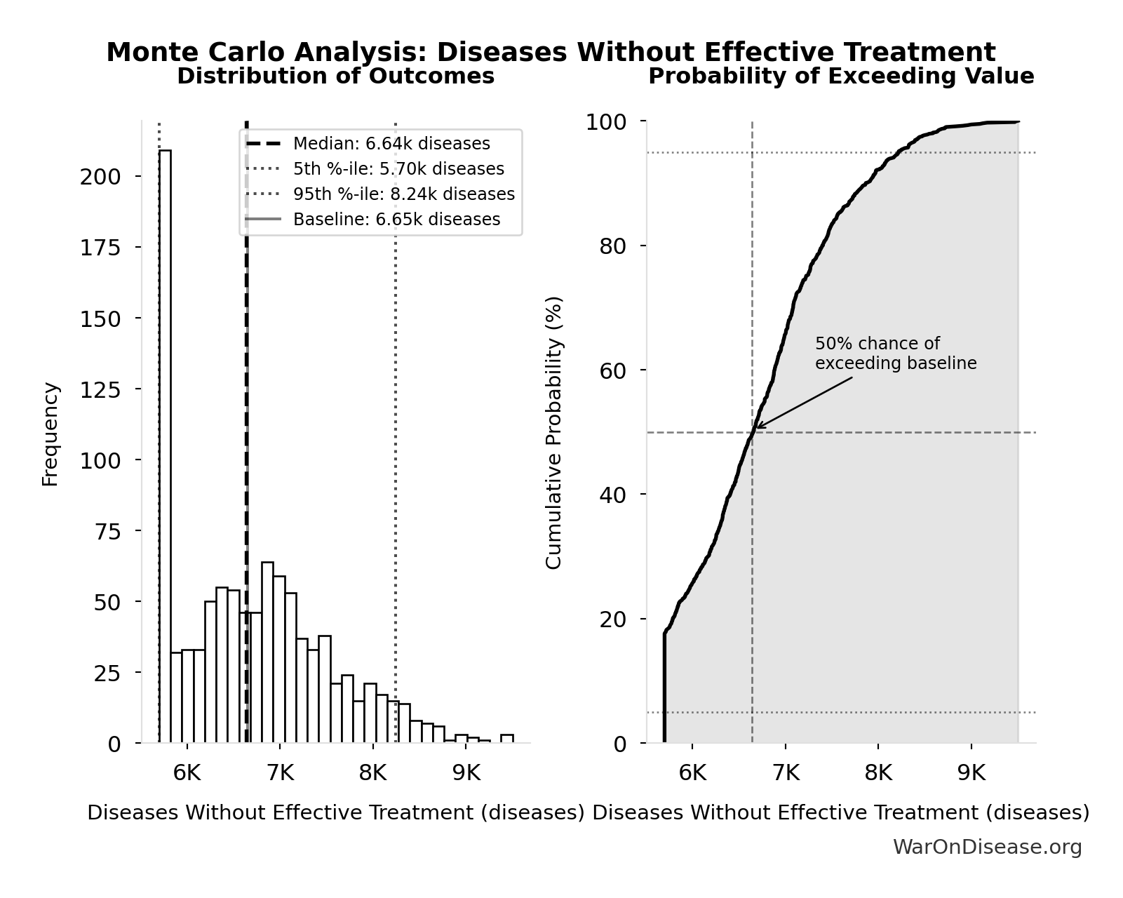
| Baseline (deterministic) | 6.65k |
| Mean (expected value) | 6.73k |
| Median (50th percentile) | 6.64k |
| Standard Deviation | 835 |
| 90% Confidence Interval | [5.70k, 8.24k] |
The histogram shows the distribution of Diseases Without Effective Treatment across 10,000 Monte Carlo simulations. The CDF (right) shows the probability of the outcome exceeding any given value, which is useful for risk assessment.
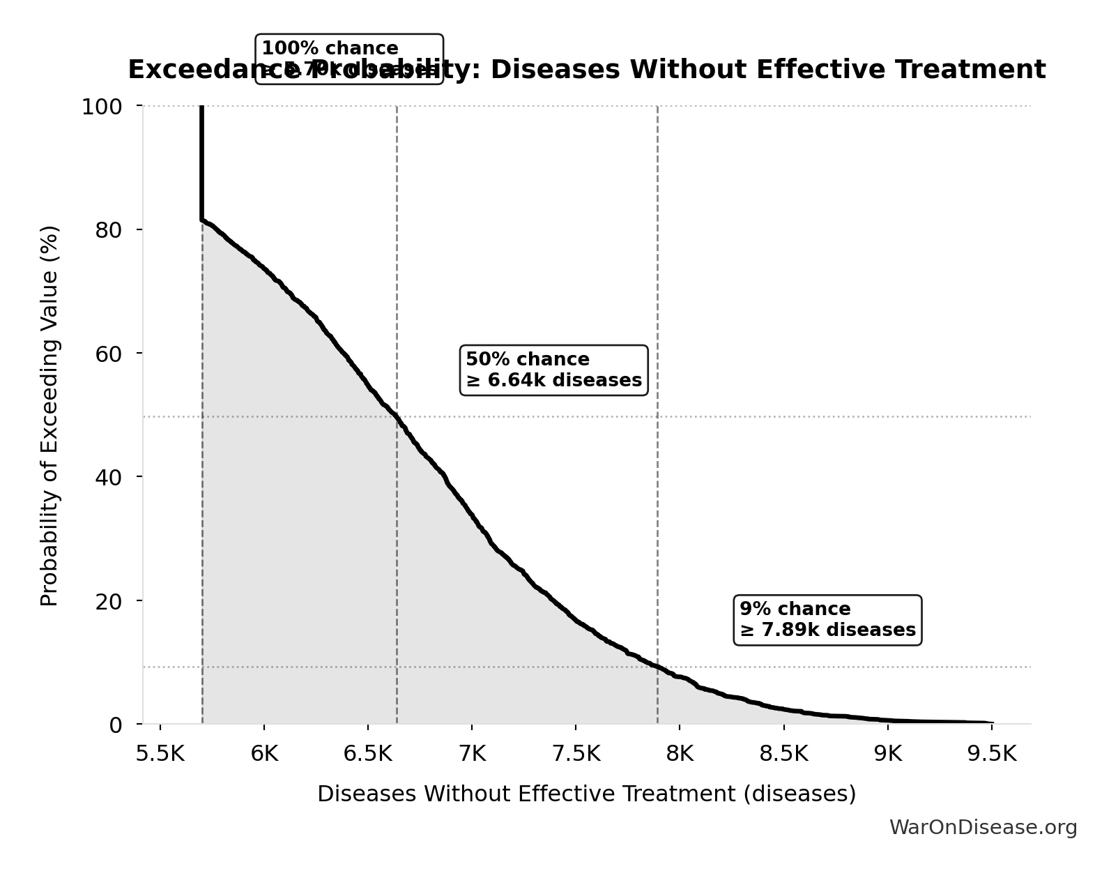
Exceedance Probability
This exceedance probability chart shows the likelihood that Diseases Without Effective Treatment will exceed any given threshold. Higher curves indicate more favorable outcomes with greater certainty.
Total Drugs Approved Since 1962: 3.10k drugs
Estimated total drugs approved globally since 1962 (62 years × average approval rate). Conservative: uses current rate, actual historical rate was lower in 1960s-80s.
Inputs:
- Average Annual New Drug Approvals Globally 📊: 50 drugs/year (95% CI: 45 drugs/year - 60 drugs/year)
\[ \begin{gathered} N_{drugs,62} \\ = Drugs_{ann,curr} \times 62 \\ = 50 \times 62 \\ = 3{,}100 \end{gathered} \]
Methodology:29
~ Medium confidence
Sensitivity Analysis
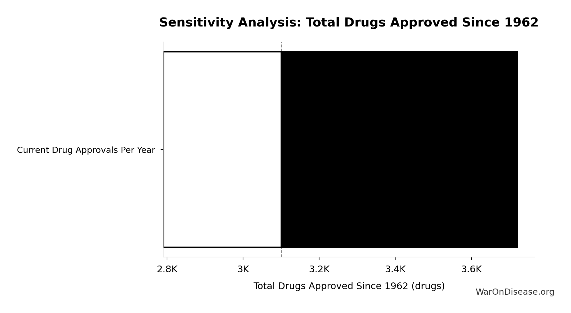
Sensitivity Indices for Total Drugs Approved Since 1962
Regression-based sensitivity showing which inputs explain the most variance in the output.
| Input Parameter | Sensitivity Coefficient | Interpretation |
|---|---|---|
| Current Drug Approvals Per Year | 1.0000 | Strong driver |
Interpretation: Standardized coefficients show the change in output (in SD units) per 1 SD change in input. Values near ±1 indicate strong influence; values exceeding ±1 may occur with correlated inputs.
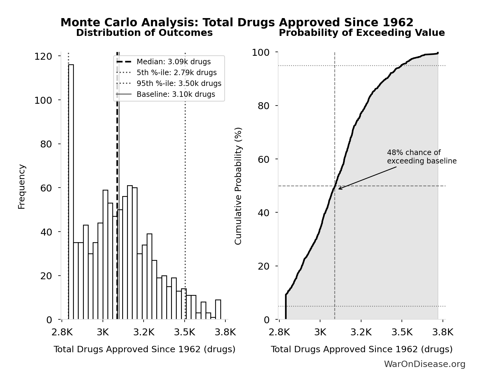
Monte Carlo Distribution
Simulation Results Summary: Total Drugs Approved Since 1962
| Statistic | Value |
|---|---|
| Baseline (deterministic) | 3.10k |
| Mean (expected value) | 3.11k |
| Median (50th percentile) | 3.09k |
| Standard Deviation | 220 |
| 90% Confidence Interval | [2.79k, 3.50k] |
The histogram shows the distribution of Total Drugs Approved Since 1962 across 10,000 Monte Carlo simulations. The CDF (right) shows the probability of the outcome exceeding any given value, which is useful for risk assessment.
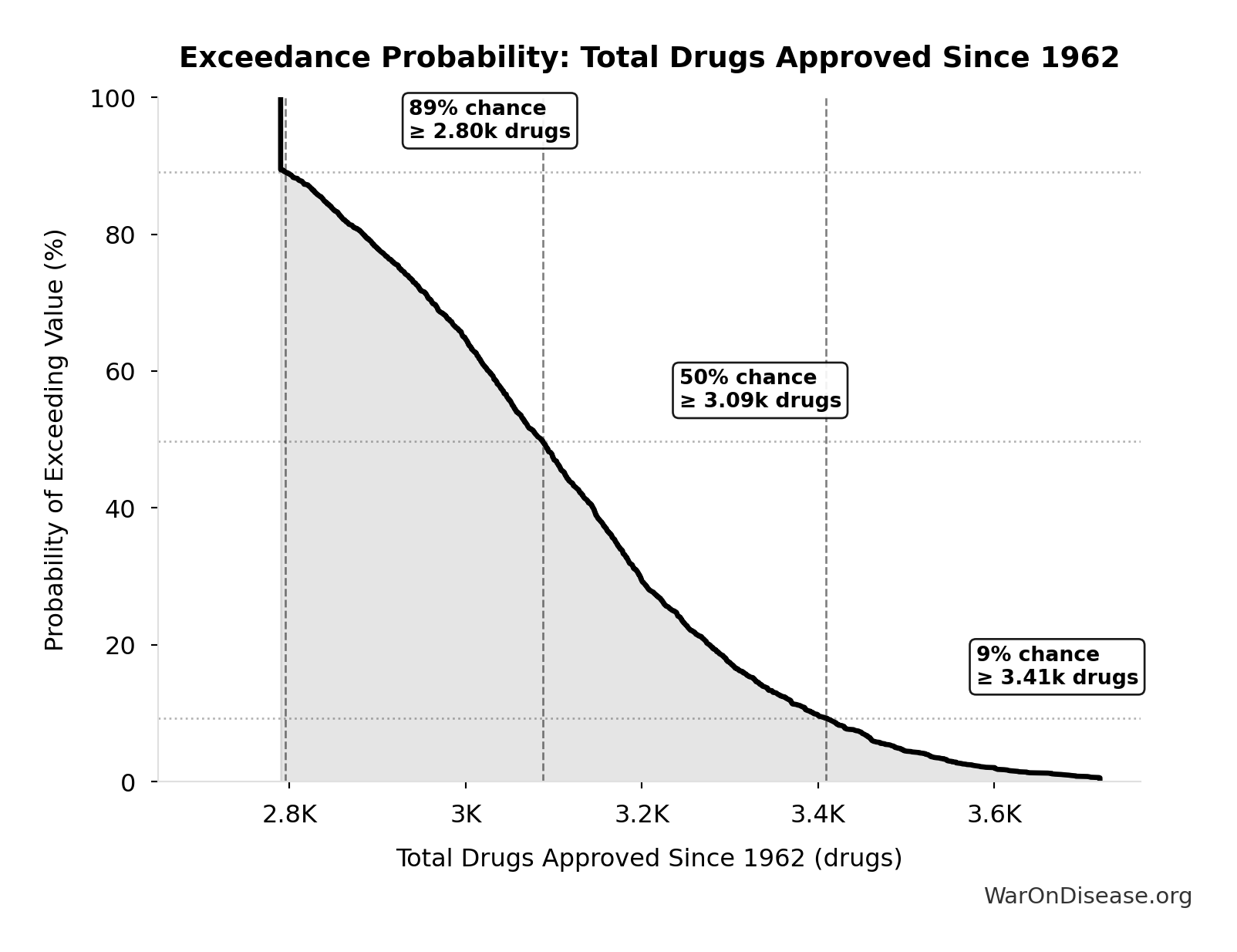
Exceedance Probability
This exceedance probability chart shows the likelihood that Total Drugs Approved Since 1962 will exceed any given threshold. Higher curves indicate more favorable outcomes with greater certainty.
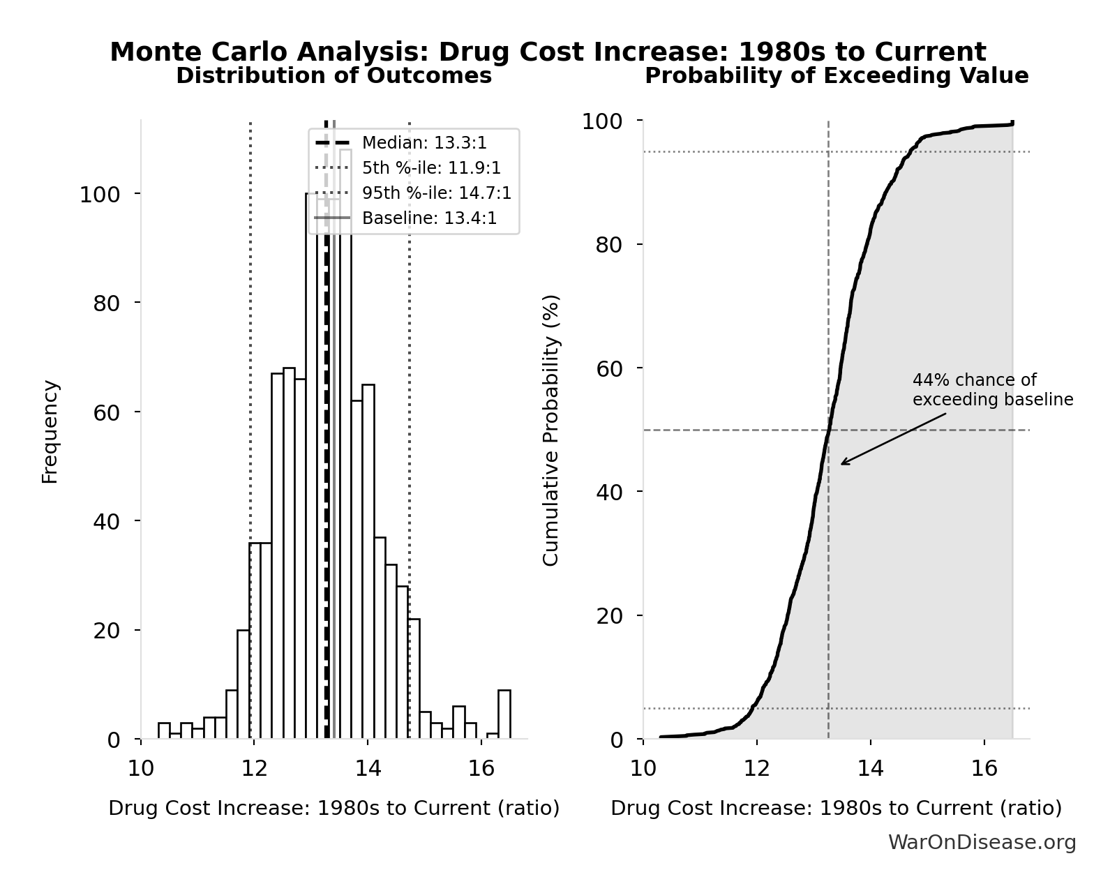
Drug Cost Increase: 1980s to Current: 13.4:1
Drug development cost increase from 1980s to current ($194M → $2.6B = 13.4x)
Inputs:
- Drug Development Cost (1980s) 📊: $194M (95% CI: $146M - $242M)
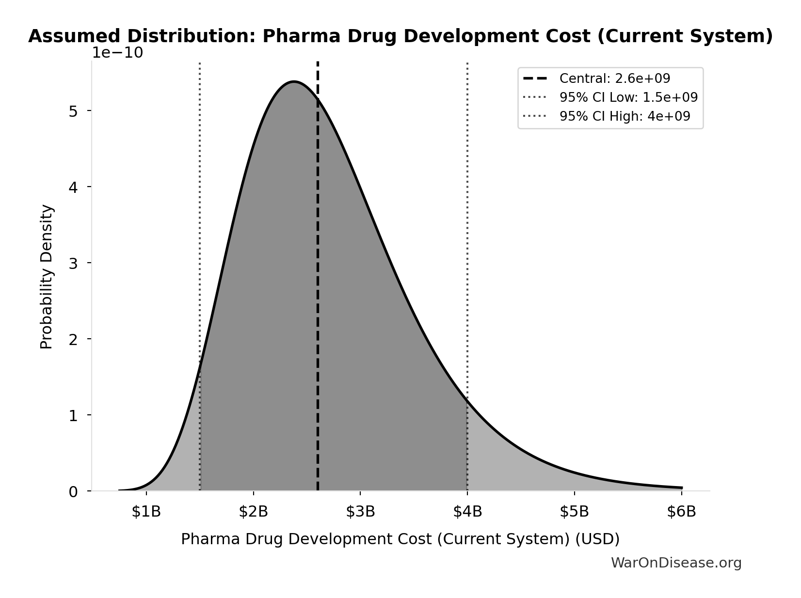
- Pharma Drug Development Cost (Current System) 📊: $2.60B (95% CI: $1.50B - $4B)
\[ \begin{gathered} k_{cost,80s} \\ = \frac{Cost_{dev,curr}}{Cost_{dev,80s}} \\ = \frac{\$2.6B}{\$194M} \\ = 13.4 \end{gathered} \]
Methodology:35
✓ High confidence
Sensitivity Analysis
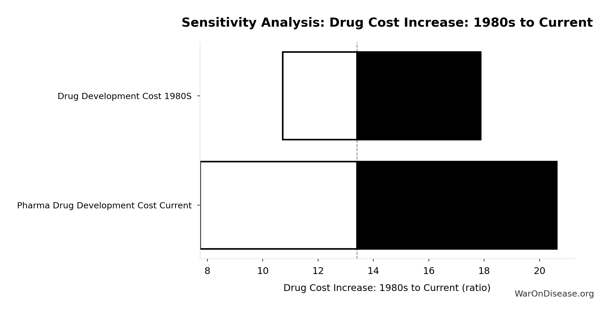
Sensitivity Indices for Drug Cost Increase: 1980s to Current
Regression-based sensitivity showing which inputs explain the most variance in the output.
| Input Parameter | Sensitivity Coefficient | Interpretation |
|---|---|---|
| Pharma Drug Development Cost Current | 1.6909 | Strong driver |
| Drug Development Cost 1980s | -0.7048 | Strong driver |
Interpretation: Standardized coefficients show the change in output (in SD units) per 1 SD change in input. Values near ±1 indicate strong influence; values exceeding ±1 may occur with correlated inputs.
Monte Carlo Distribution
Simulation Results Summary: Drug Cost Increase: 1980s to Current
| Statistic | Value |
|---|---|
| Baseline (deterministic) | 13.4:1 |
| Mean (expected value) | 13.3:1 |
| Median (50th percentile) | 13.3:1 |
| Standard Deviation | 0.915:1 |
| 90% Confidence Interval | [11.9:1, 14.7:1] |
The histogram shows the distribution of Drug Cost Increase: 1980s to Current across 10,000 Monte Carlo simulations. The CDF (right) shows the probability of the outcome exceeding any given value, which is useful for risk assessment.
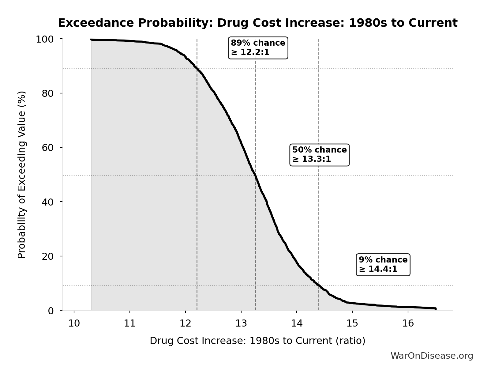
Exceedance Probability
This exceedance probability chart shows the likelihood that Drug Cost Increase: 1980s to Current will exceed any given threshold. Higher curves indicate more favorable outcomes with greater certainty.
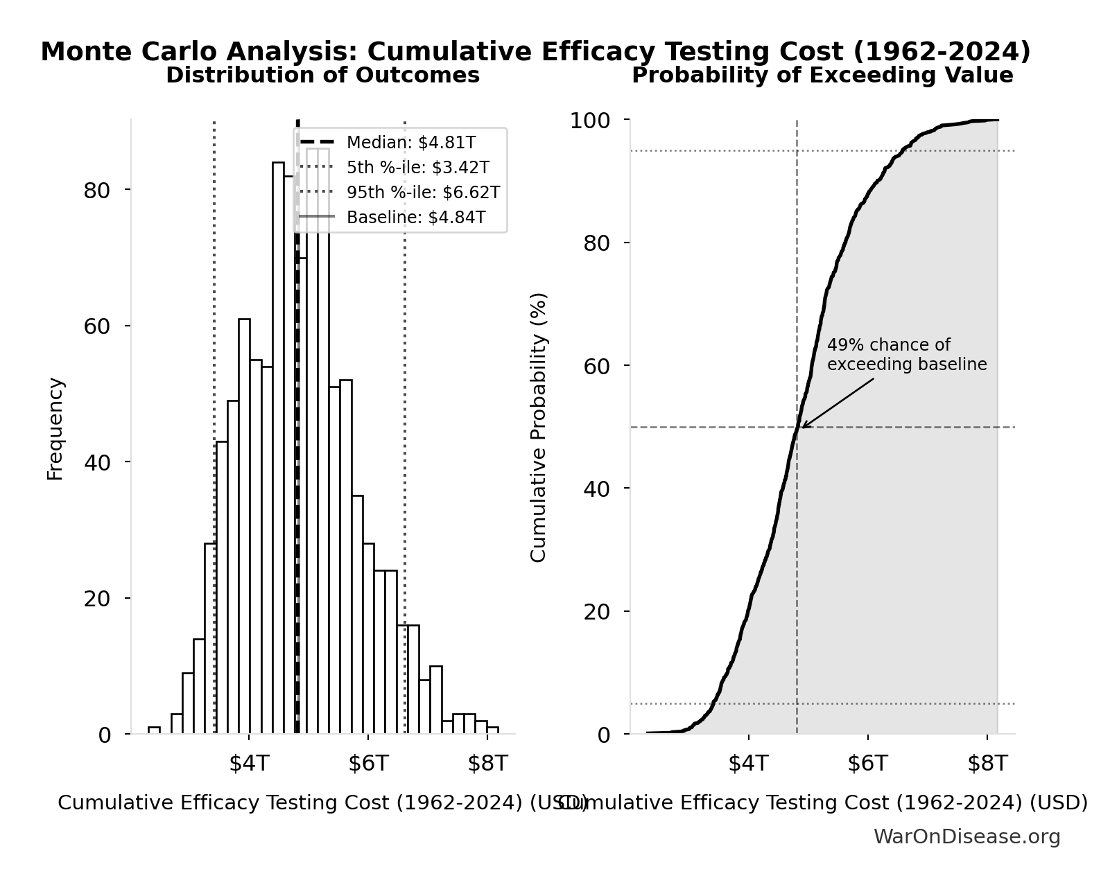
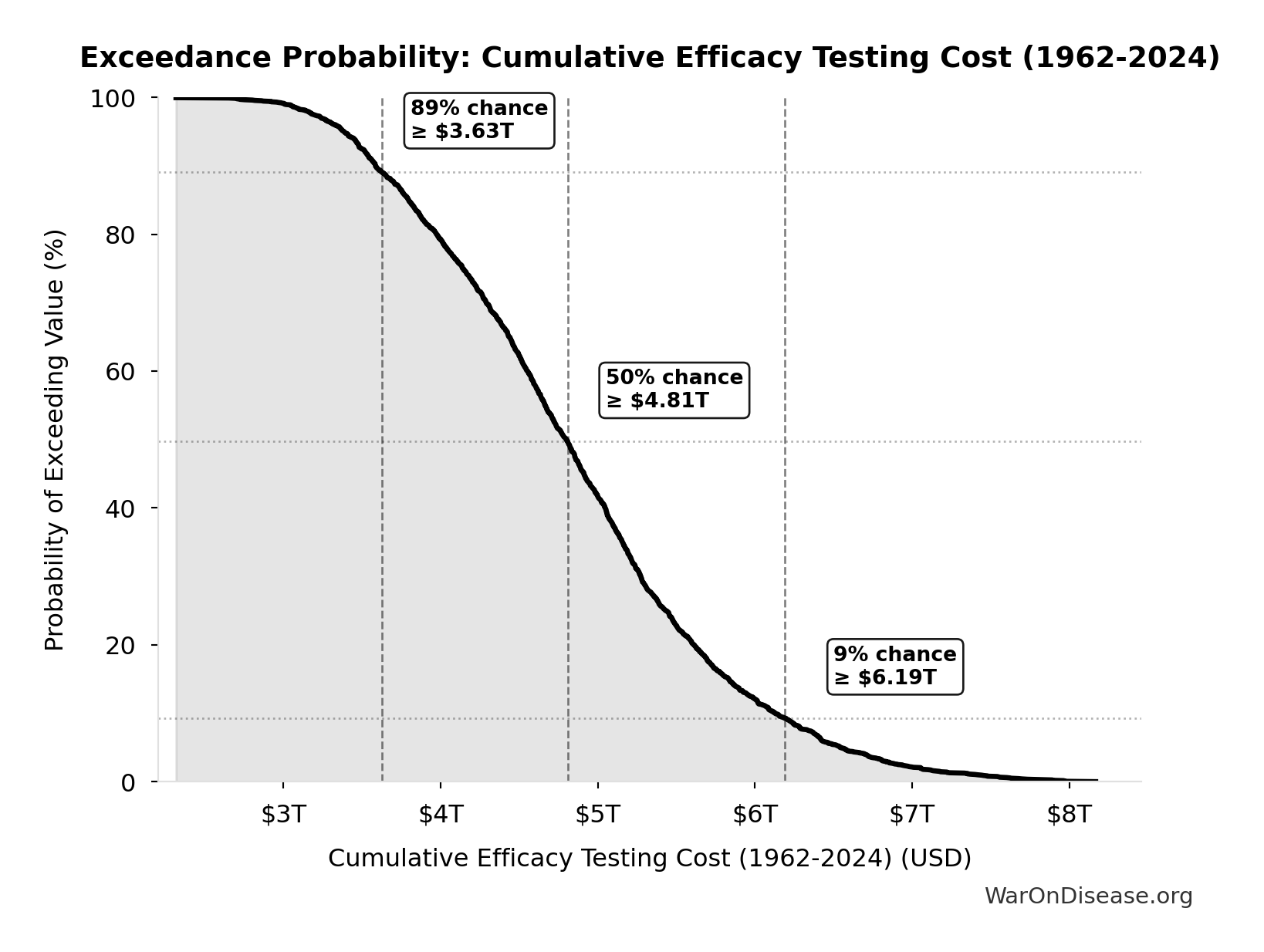
Cumulative Efficacy Testing Cost (1962-2024): $4.84T
Cumulative Phase 2/3 efficacy testing cost since 1962. Uses direct Phase 2/3 cost ($1.56B per drug) - this is a LOWER BOUND because it excludes opportunity cost of 8.2-year delays, compounds abandoned due to cost barrier, and regulatory overhead. Comparable to the $8 trillion spent on post-9/11 wars.
Inputs:
- Pharma Phase 2/3 Cost Barrier Per Drug: $1.56B (SE: ±$200M)
- Total Drugs Approved Since 1962 🔢: 3.10k drugs
\[ \begin{gathered} Cost_{eff,cumul} \\ = Cost_{P2+P3} \times N_{drugs,62} \\ = \$1.56B \times 3{,}100 \\ = \$4.84T \\[0.5em] \text{where } N_{drugs,62} = Drugs_{ann,curr} \times 62 = 50 \times 62 = 3{,}100 \end{gathered} \]
Methodology: ../appendix/invisible-graveyard#scale
~ Medium confidence
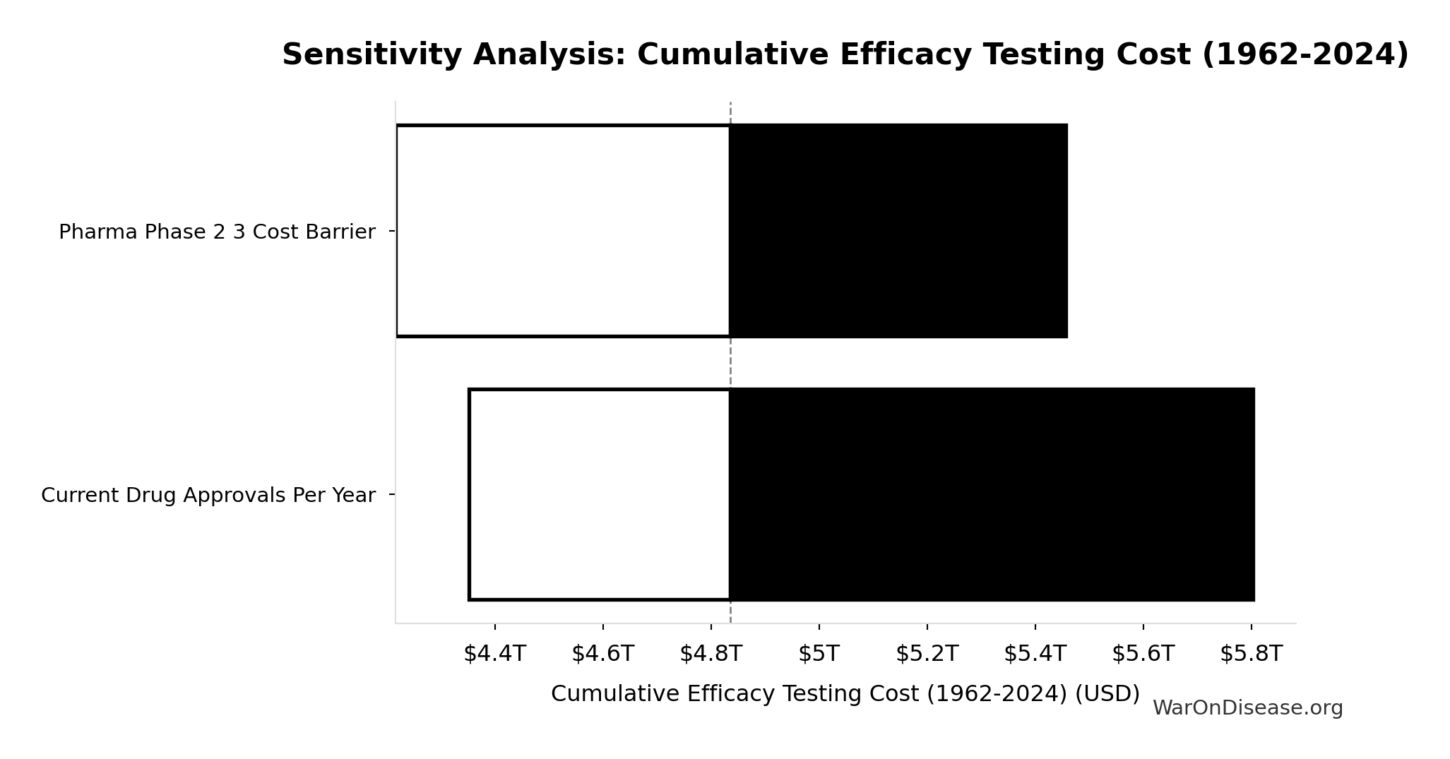
Sensitivity Analysis
Sensitivity Indices for Cumulative Efficacy Testing Cost (1962-2024)
Regression-based sensitivity showing which inputs explain the most variance in the output.
| Input Parameter | Sensitivity Coefficient | Interpretation |
|---|---|---|
| Drugs Approved Since 1962 | 0.5385 | Strong driver |
| Pharma Phase 2 3 Cost Barrier | 0.4652 | Moderate driver |
Interpretation: Standardized coefficients show the change in output (in SD units) per 1 SD change in input. Values near ±1 indicate strong influence; values exceeding ±1 may occur with correlated inputs.
Monte Carlo Distribution
Simulation Results Summary: Cumulative Efficacy Testing Cost (1962-2024)
| Statistic | Value |
|---|---|
| Baseline (deterministic) | $4.84T |
| Mean (expected value) | $4.88T |
| Median (50th percentile) | $4.81T |
| Standard Deviation | $977B |
| 90% Confidence Interval | [$3.42T, $6.62T] |
The histogram shows the distribution of Cumulative Efficacy Testing Cost (1962-2024) across 10,000 Monte Carlo simulations. The CDF (right) shows the probability of the outcome exceeding any given value, which is useful for risk assessment.
Exceedance Probability
This exceedance probability chart shows the likelihood that Cumulative Efficacy Testing Cost (1962-2024) will exceed any given threshold. Higher curves indicate more favorable outcomes with greater certainty.
Efficacy Lag Deaths (9/11 Equivalents): 34.1k 9/11s
Total deaths from efficacy lag expressed in 9/11 equivalents. Makes the mortality cost viscerally understandable: how many September 11ths worth of deaths did the 1962 efficacy requirements cause?
Inputs:
- Total Deaths from Historical Progress Delays 🔢: 102M deaths
- September 11 Deaths 📊: 2.98k people
\[ \begin{gathered} N_{9/11,equiv} = \frac{Deaths_{lag,total}}{N_{9/11}} = \frac{102M}{2{,}980} = 34{,}100 \\[0.5em] \text{where } Deaths_{lag,total} \\ = Lives_{saved,annual} \times T_{lag} \\ = 12.4M \times 8.2 \\ = 102M \\[0.5em] \text{where } Lives_{saved,annual} = \frac{LY_{saved,annual}}{T_{ext}} = \frac{149M}{12} = 12.4M \end{gathered} \]
Methodology: ../appendix/invisible-graveyard#scale
~ Medium confidence
Sensitivity Analysis
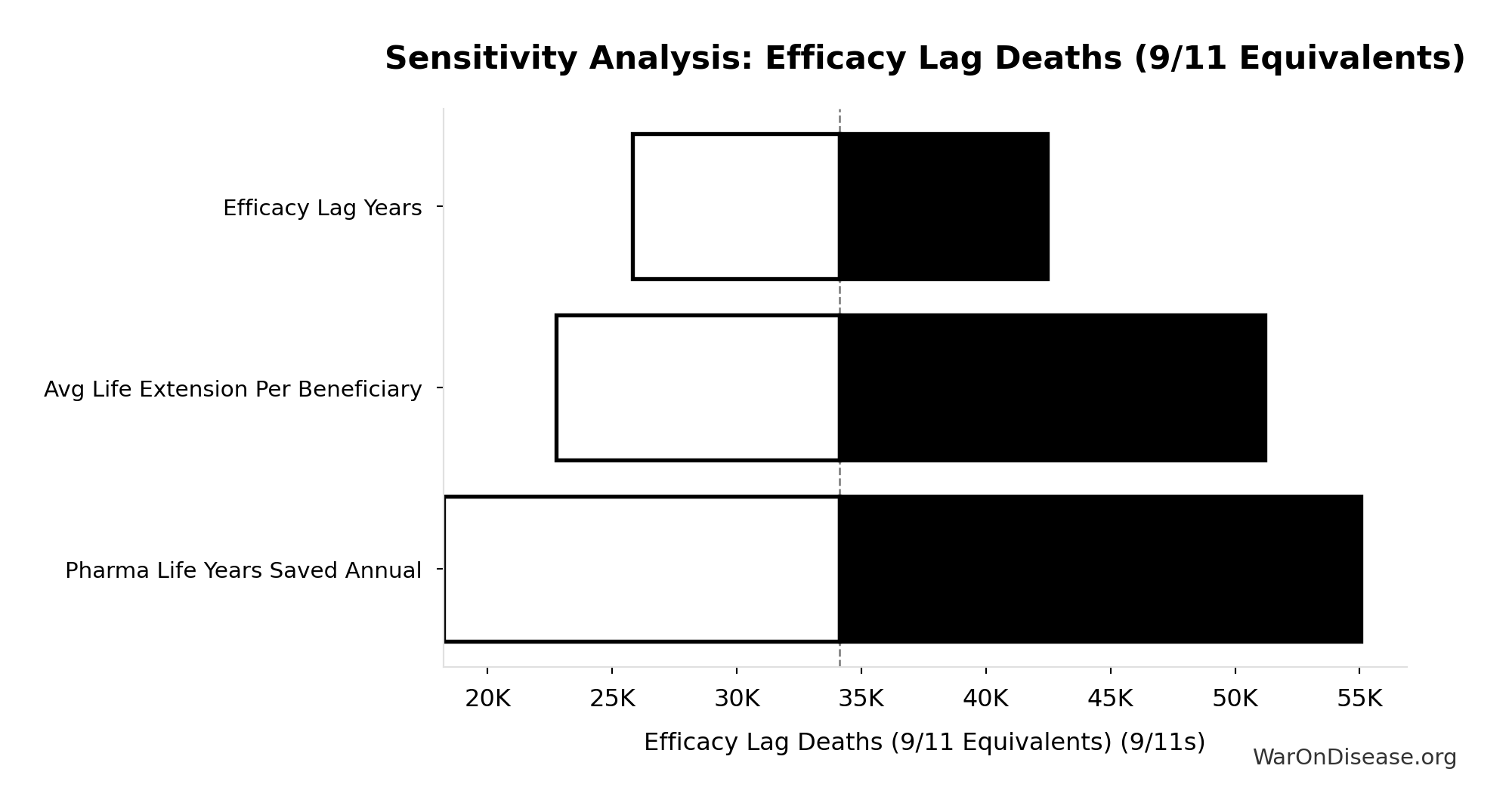
Sensitivity Indices for Efficacy Lag Deaths (9/11 Equivalents)
Regression-based sensitivity showing which inputs explain the most variance in the output.
| Input Parameter | Sensitivity Coefficient | Interpretation |
|---|---|---|
| Existing Drugs Efficacy Lag Deaths Total | 1.0000 | Strong driver |
Interpretation: Standardized coefficients show the change in output (in SD units) per 1 SD change in input. Values near ±1 indicate strong influence; values exceeding ±1 may occur with correlated inputs.
Monte Carlo Distribution
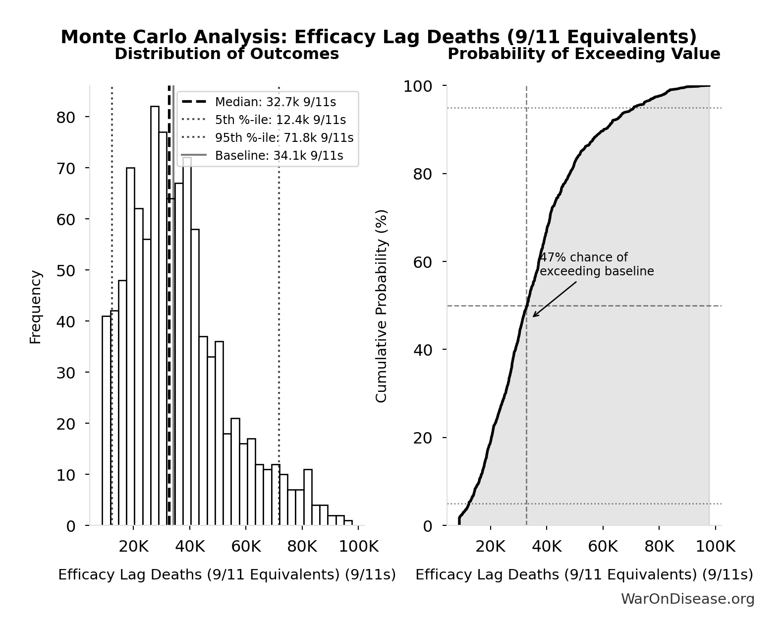
Simulation Results Summary: Efficacy Lag Deaths (9/11 Equivalents)
| Statistic | Value |
|---|---|
| Baseline (deterministic) | 34.1k |
| Mean (expected value) | 36.0k |
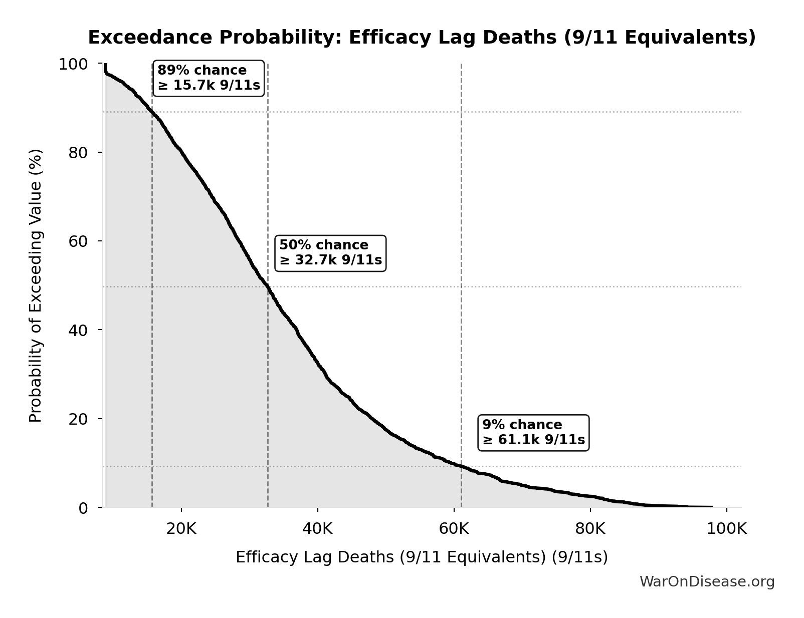
| Median (50th percentile) | 32.7k |
| Standard Deviation | 17.8k |
| 90% Confidence Interval | [12.4k, 71.8k] |
The histogram shows the distribution of Efficacy Lag Deaths (9/11 Equivalents) across 10,000 Monte Carlo simulations. The CDF (right) shows the probability of the outcome exceeding any given value, which is useful for risk assessment.
Exceedance Probability
This exceedance probability chart shows the likelihood that Efficacy Lag Deaths (9/11 Equivalents) will exceed any given threshold. Higher curves indicate more favorable outcomes with greater certainty.
Treatment Delay YLD - Annual: 2.01B DALYs
Annual YLD from treatment delay: patients receiving chronic disease treatment would have collectively avoided this disability if treatments were available 8.2 years earlier. Represents morbidity burden for treatment beneficiaries (distinct from mortality burden).
Inputs:
- Annual Chronic Disease Patients Treated 🔢: 982M people
- Regulatory Delay for Efficacy Testing Post-Safety Verification 📊: 8.2 years (SE: ±2 years)
- Treatment Disability Reduction 📊: 0.25 weight (95% CI: 0.15 weight - 0.35 weight)
\[ \begin{gathered} YLD_{treat\_delay} \\ = N_{treated} \times T_{lag} \times \Delta DW_{treat} \\ = 982M \times 8.2 \times 0.25 \\ = 2.01B \\[0.5em] \text{where } N_{treated} \\ = DOT_{chronic} \times 0.000767 \\ = 1.28T \times 0.000767 \\ = 982M \end{gathered} \]
Methodology: ../appendix/invisible-graveyard#treatment-morbidity
? Low confidence
Sensitivity Analysis
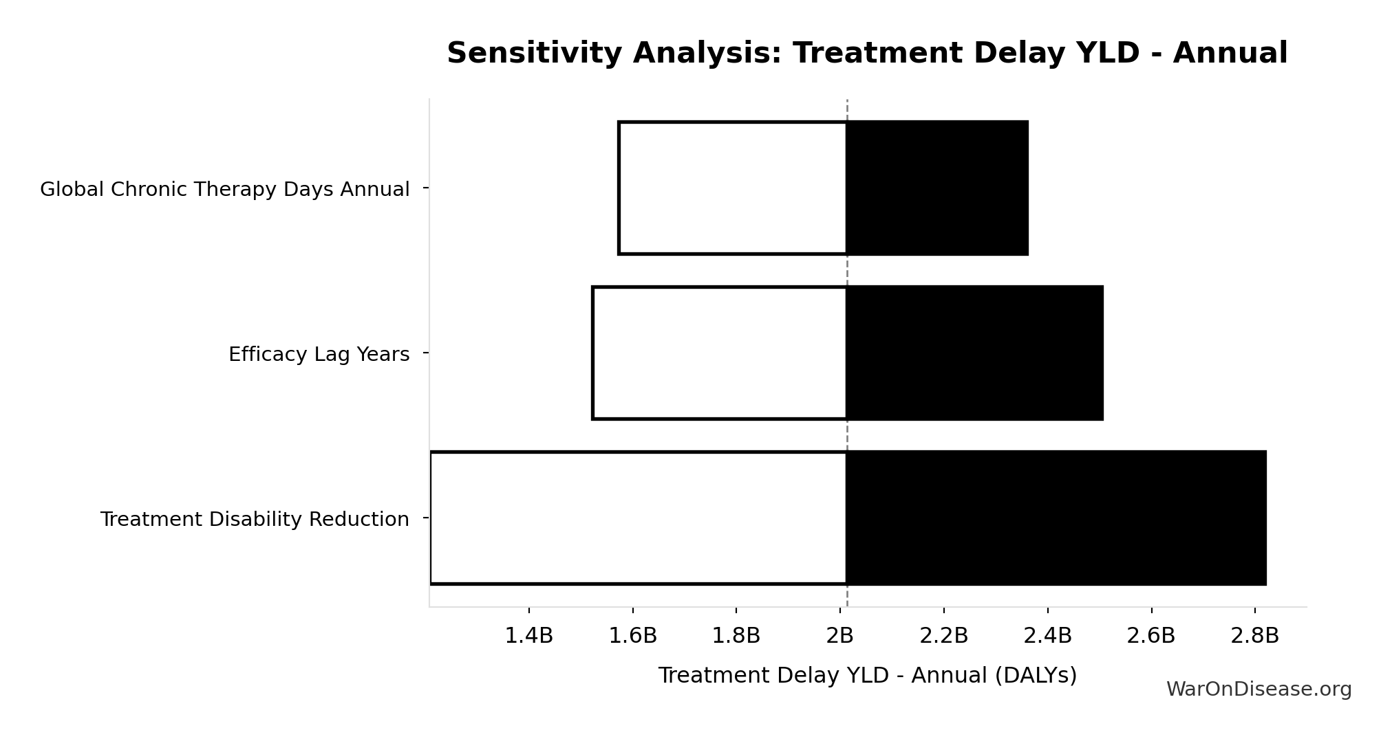
Sensitivity Indices for Treatment Delay YLD - Annual
Regression-based sensitivity showing which inputs explain the most variance in the output.
| Input Parameter | Sensitivity Coefficient | Interpretation |
|---|---|---|
| Chronic Disease Treated Patients Annual | 3.0959 | Strong driver |
| Treatment Disability Reduction | -2.4506 | Strong driver |
| Efficacy Lag Years | 0.3319 | Moderate driver |
Interpretation: Standardized coefficients show the change in output (in SD units) per 1 SD change in input. Values near ±1 indicate strong influence; values exceeding ±1 may occur with correlated inputs.
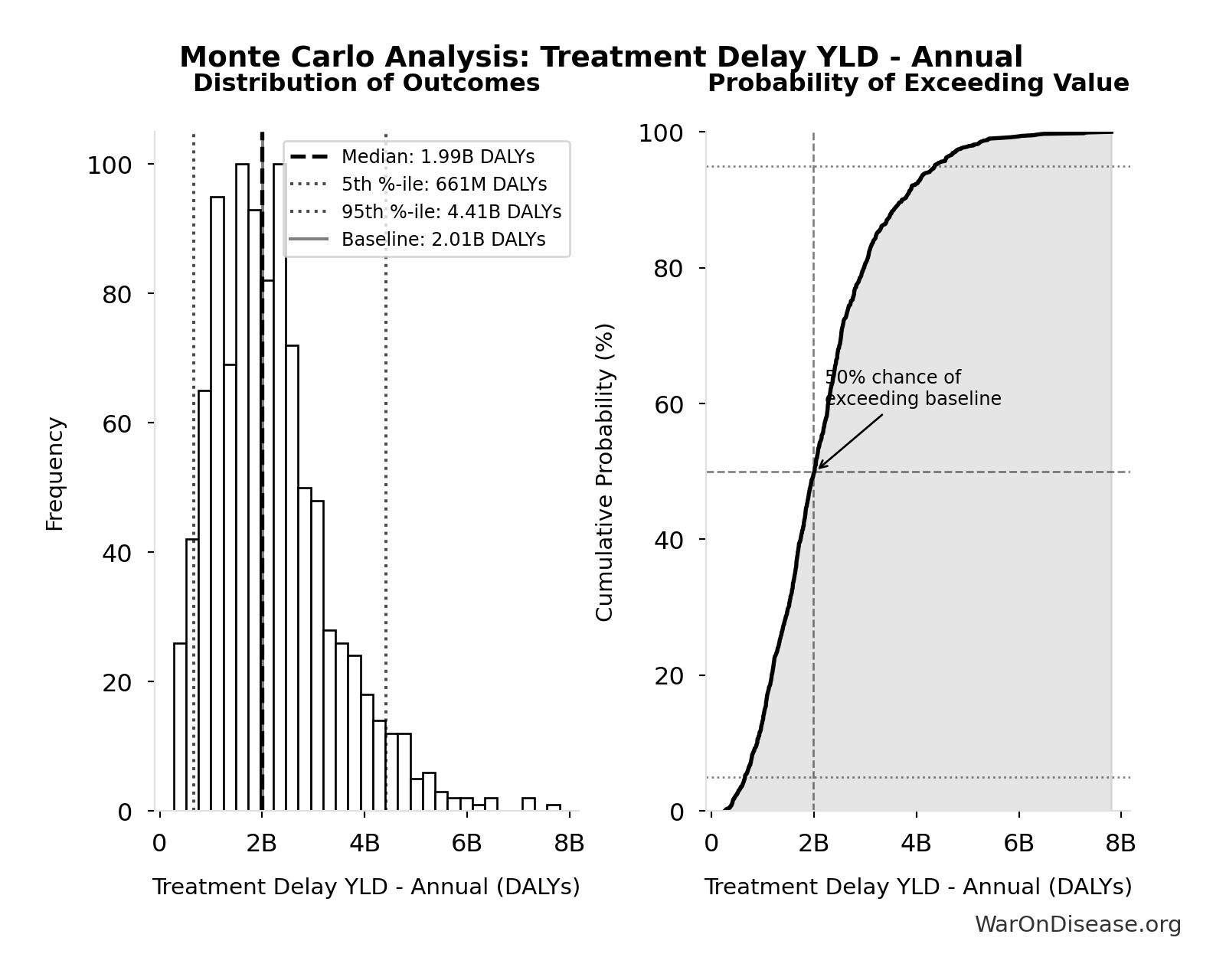
Monte Carlo Distribution
Simulation Results Summary: Treatment Delay YLD - Annual
| Statistic | Value |
|---|---|
| Baseline (deterministic) | 2.01B |
| Mean (expected value) | 2.20B |
| Median (50th percentile) | 1.99B |
| Standard Deviation | 1.18B |
| 90% Confidence Interval | [661M, 4.41B] |
The histogram shows the distribution of Treatment Delay YLD - Annual across 10,000 Monte Carlo simulations. The CDF (right) shows the probability of the outcome exceeding any given value, which is useful for risk assessment.
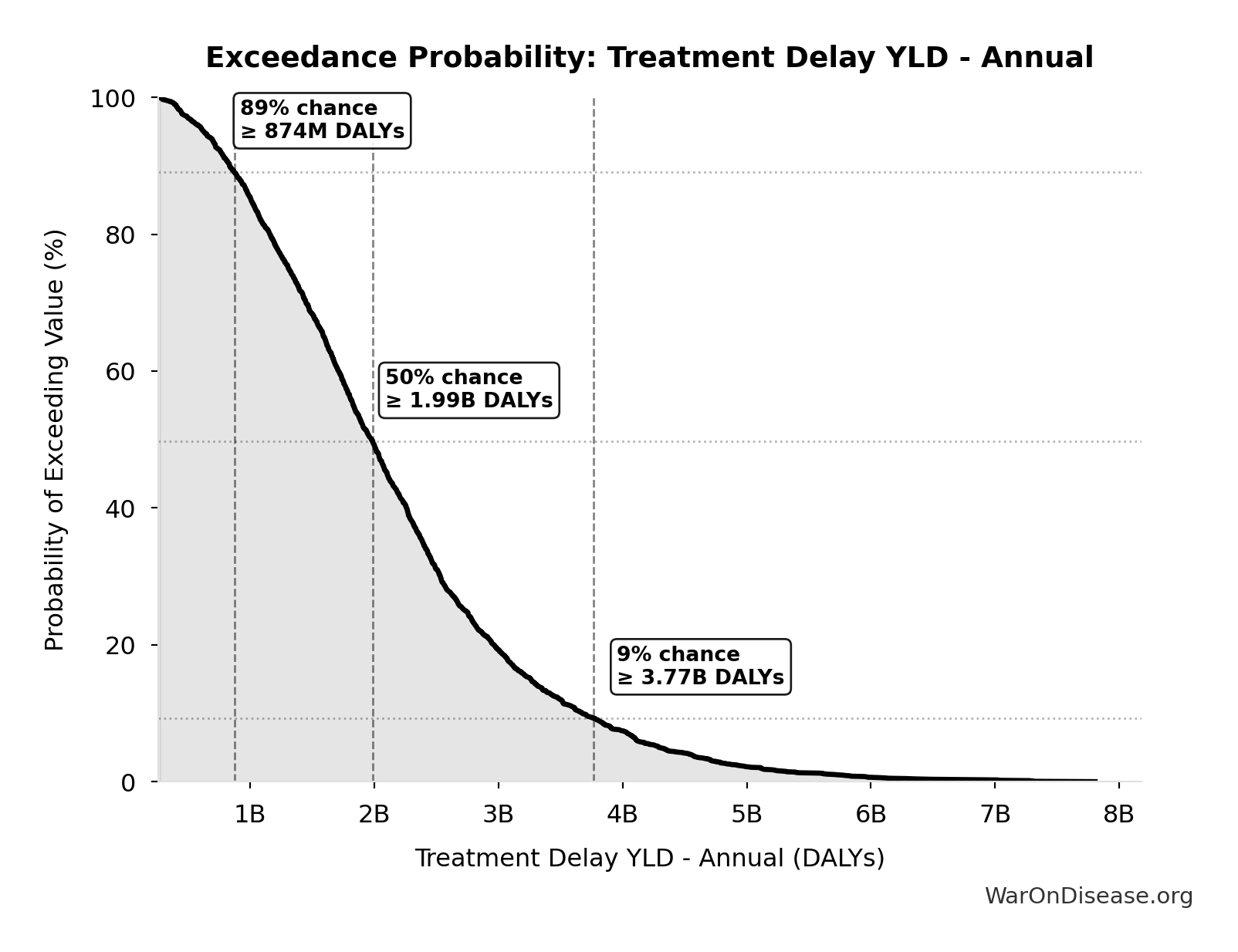
Exceedance Probability
This exceedance probability chart shows the likelihood that Treatment Delay YLD - Annual will exceed any given threshold. Higher curves indicate more favorable outcomes with greater certainty.
Total Deaths from Historical Progress Delays: 102M deaths
Total deaths from delaying existing drugs over 8.2-year efficacy lag. One-time impact of eliminating Phase 2-4 testing delay for drugs already approved 1962-2024. Based on Lichtenberg (2019) estimate of 12M lives saved annually × 8.2 years efficacy lag. Excludes innovation acceleration effects.
Inputs:
- Annual Lives Saved by Pharmaceuticals 🔢: 12.4M deaths
- Regulatory Delay for Efficacy Testing Post-Safety Verification 📊: 8.2 years (SE: ±2 years)
\[ \begin{gathered} Deaths_{lag,total} \\ = Lives_{saved,annual} \times T_{lag} \\ = 12.4M \times 8.2 \\ = 102M \\[0.5em] \text{where } Lives_{saved,annual} = \frac{LY_{saved,annual}}{T_{ext}} = \frac{149M}{12} = 12.4M \end{gathered} \]
Methodology: ../appendix/invisible-graveyard#historical-progress
~ Medium confidence
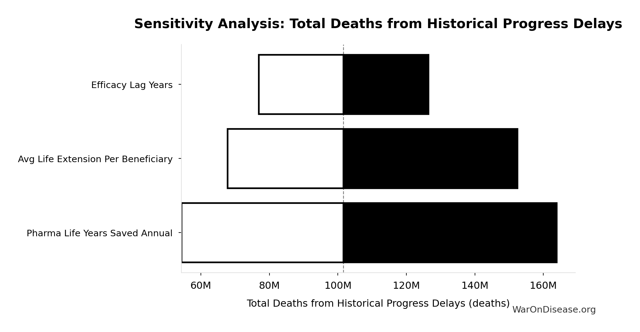
Sensitivity Analysis
Sensitivity Indices for Total Deaths from Historical Progress Delays
Regression-based sensitivity showing which inputs explain the most variance in the output.
| Input Parameter | Sensitivity Coefficient | Interpretation |
|---|---|---|
| Pharma Lives Saved Annual | 1.2721 | Strong driver |
| Efficacy Lag Years | -0.2811 | Weak driver |
Interpretation: Standardized coefficients show the change in output (in SD units) per 1 SD change in input. Values near ±1 indicate strong influence; values exceeding ±1 may occur with correlated inputs.
Monte Carlo Distribution
Simulation Results Summary: Total Deaths from Historical Progress Delays
| Statistic | Value |
|---|---|
| Baseline (deterministic) | 102M |
| Mean (expected value) | 107M |
| Median (50th percentile) | 97.3M |
| Standard Deviation | 53.0M |
| 90% Confidence Interval | [36.9M, 214M] |
The histogram shows the distribution of Total Deaths from Historical Progress Delays across 10,000 Monte Carlo simulations. The CDF (right) shows the probability of the outcome exceeding any given value, which is useful for risk assessment.
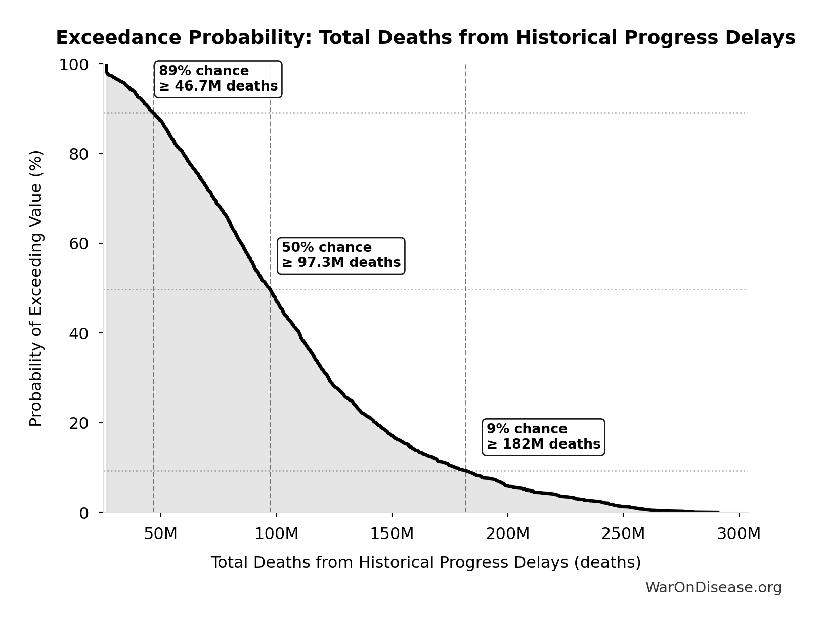
Exceedance Probability
This exceedance probability chart shows the likelihood that Total Deaths from Historical Progress Delays will exceed any given threshold. Higher curves indicate more favorable outcomes with greater certainty.
Annual Lives Saved by Pharmaceuticals: 12.4M deaths
Annual lives saved by pharmaceutical interventions globally. Derived from Lichtenberg (2019) finding of 148.7M life-years saved, divided by assumed 12-year average life extension per beneficiary. Note: Life-years is the primary metric; lives is an approximation for intuitive communication.
Inputs:
- Annual Life-Years Saved by Pharmaceuticals 📊: 149M life-years (95% CI: 79.4M life-years - 240M life-years)
- Average Life Extension per Beneficiary: 12 years (95% CI: 8 years - 18 years)
\[ \begin{gathered} Lives_{saved,annual} \\ = \frac{LY_{saved,annual}}{T_{ext}} \\ = \frac{149M}{12} \\ = 12.4M \end{gathered} \]
Methodology:84
? Low confidence
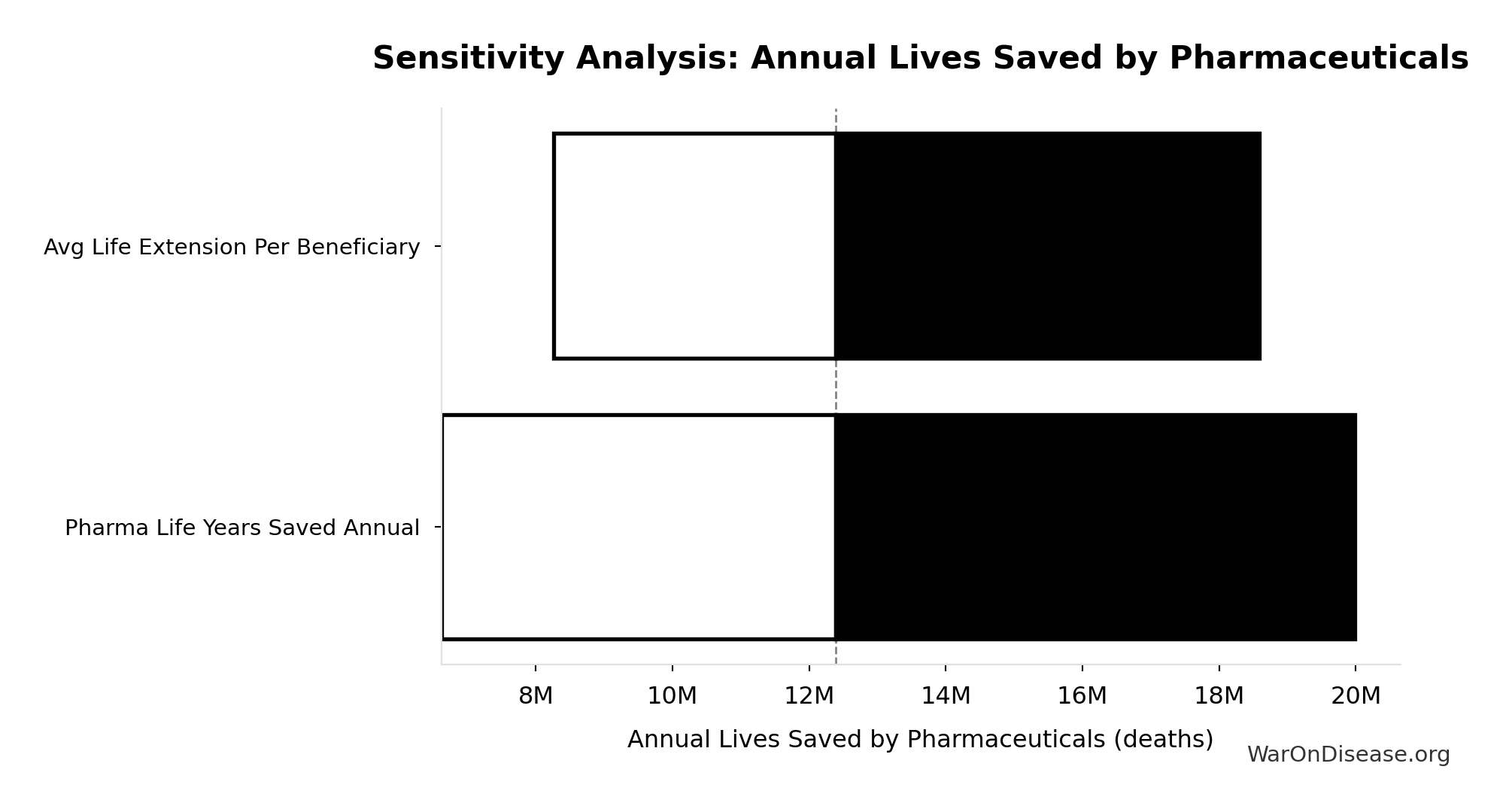
Sensitivity Analysis
Sensitivity Indices for Annual Lives Saved by Pharmaceuticals
Regression-based sensitivity showing which inputs explain the most variance in the output.
| Input Parameter | Sensitivity Coefficient | Interpretation |
|---|---|---|
| Pharma Life Years Saved Annual | 1.0000 | Strong driver |
Interpretation: Standardized coefficients show the change in output (in SD units) per 1 SD change in input. Values near ±1 indicate strong influence; values exceeding ±1 may occur with correlated inputs.
Monte Carlo Distribution
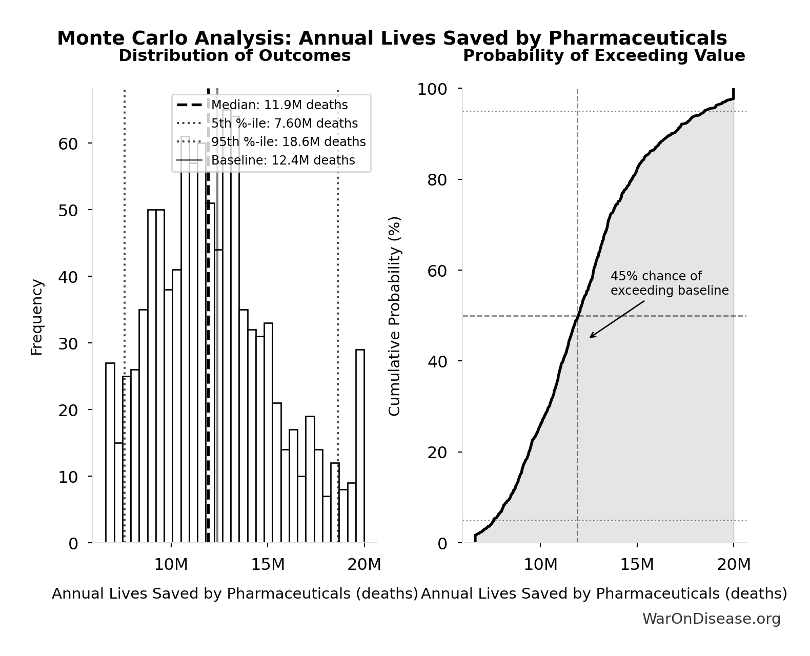
Simulation Results Summary: Annual Lives Saved by Pharmaceuticals
| Statistic | Value |
|---|---|
| Baseline (deterministic) | 12.4M |
| Mean (expected value) | 12.3M |
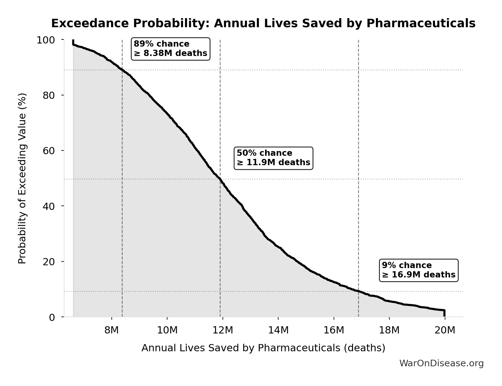
| Median (50th percentile) | 11.9M |
| Standard Deviation | 3.20M |
| 90% Confidence Interval | [7.60M, 18.6M] |
The histogram shows the distribution of Annual Lives Saved by Pharmaceuticals across 10,000 Monte Carlo simulations. The CDF (right) shows the probability of the outcome exceeding any given value, which is useful for risk assessment.
Exceedance Probability
This exceedance probability chart shows the likelihood that Annual Lives Saved by Pharmaceuticals will exceed any given threshold. Higher curves indicate more favorable outcomes with greater certainty.
Thalidomide DALYs Per Event: 41.8k DALYs
Total DALYs per US-scale thalidomide event (YLL + YLD)
Inputs:
- Thalidomide YLD Per Event 🔢: 13.0k years
- Thalidomide YLL Per Event 🔢: 28.8k years
\[ \begin{gathered} DALY_{thal} \\ = YLD_{thal} + YLL_{thal} \\ = 13{,}000 + 28{,}800 \\ = 41{,}800 \\[0.5em] \text{where } YLD_{thal} \\ = DW_{thal} \times N_{thal,survive} \times LE_{thal} \\ = 0.4 \times 540 \times 60 \\ = 13{,}000 \\[0.5em] \text{where } N_{thal,survive} \\ = N_{thal,US,prevent} \times (1 - Rate_{thal,mort}) \\ = 900 \times (1 - 40\%) \\ = 540 \\[0.5em] \text{where } N_{thal,US,prevent} \\ = N_{thal,global} \times Pct_{US,1960} \\ = 15{,}000 \times 6\% \\ = 900 \\[0.5em] \text{where } YLL_{thal} = Deaths_{thal} \times 80 = 360 \times 80 = 28{,}800 \\[0.5em] \text{where } Deaths_{thal} \\ = Rate_{thal,mort} \times N_{thal,US,prevent} \\ = 40\% \times 900 \\ = 360 \\[0.5em] \text{where } N_{thal,US,prevent} \\ = N_{thal,global} \times Pct_{US,1960} \\ = 15{,}000 \times 6\% \\ = 900 \end{gathered} \]
~ Medium confidence
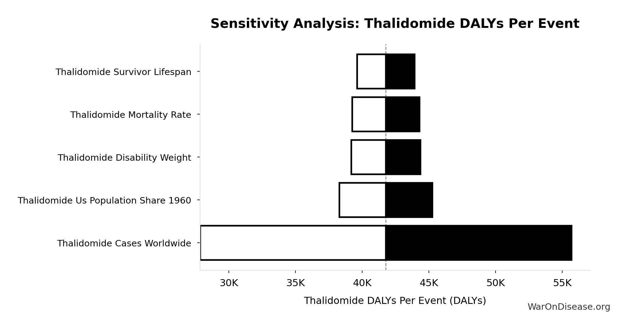
Sensitivity Analysis
Sensitivity Indices for Thalidomide DALYs Per Event
Regression-based sensitivity showing which inputs explain the most variance in the output.
| Input Parameter | Sensitivity Coefficient | Interpretation |
|---|---|---|
| Thalidomide Yll Per Event | 0.6300 | Strong driver |
| Thalidomide Yld Per Event | 0.3701 | Moderate driver |
Interpretation: Standardized coefficients show the change in output (in SD units) per 1 SD change in input. Values near ±1 indicate strong influence; values exceeding ±1 may occur with correlated inputs.
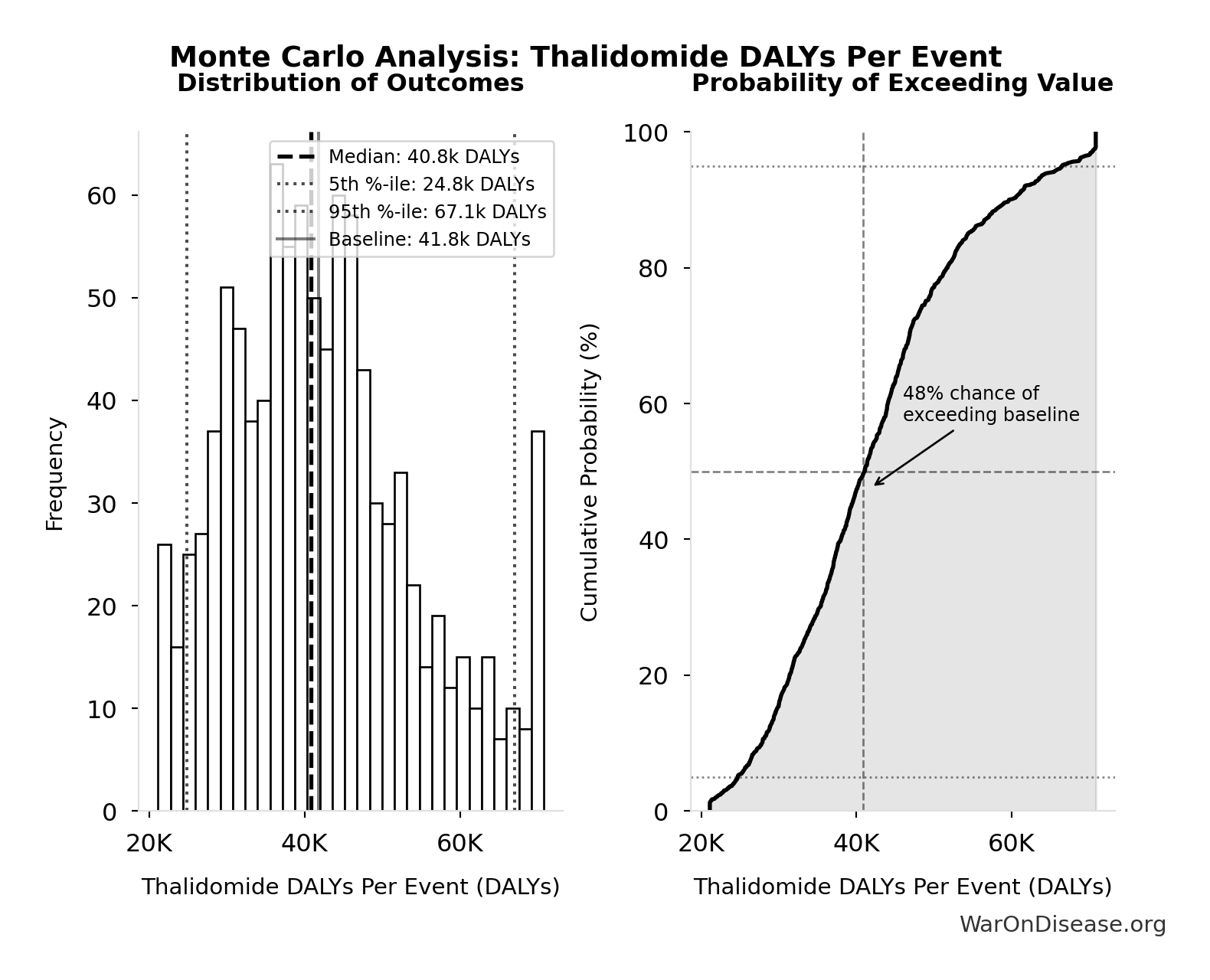
Monte Carlo Distribution
Simulation Results Summary: Thalidomide DALYs Per Event
| Statistic | Value |
|---|---|
| Baseline (deterministic) | 41.8k |
| Mean (expected value) | 42.5k |
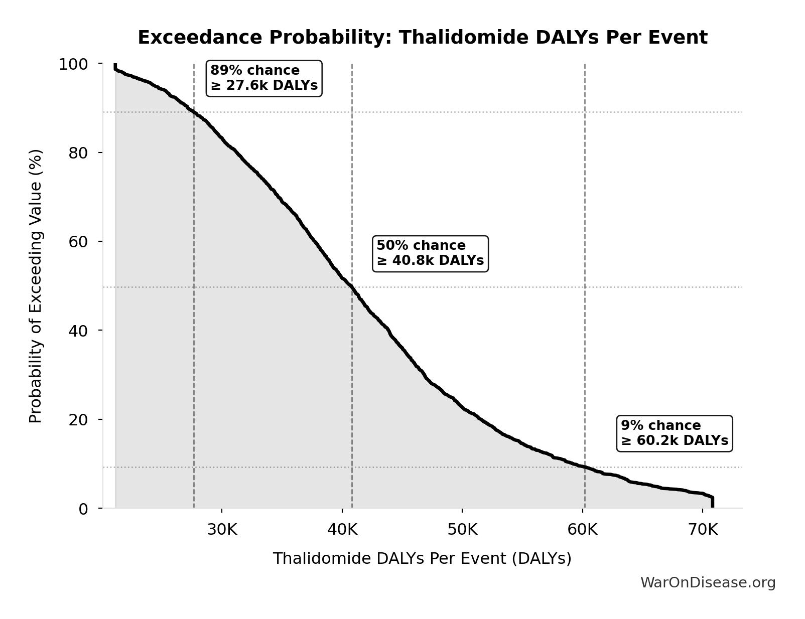
| Median (50th percentile) | 40.8k |
| Standard Deviation | 12.2k |
| 90% Confidence Interval | [24.8k, 67.1k] |
The histogram shows the distribution of Thalidomide DALYs Per Event across 10,000 Monte Carlo simulations. The CDF (right) shows the probability of the outcome exceeding any given value, which is useful for risk assessment.
Exceedance Probability
This exceedance probability chart shows the likelihood that Thalidomide DALYs Per Event will exceed any given threshold. Higher curves indicate more favorable outcomes with greater certainty.
Thalidomide Deaths Per Event: 360 deaths
Deaths per US-scale thalidomide event
Inputs:
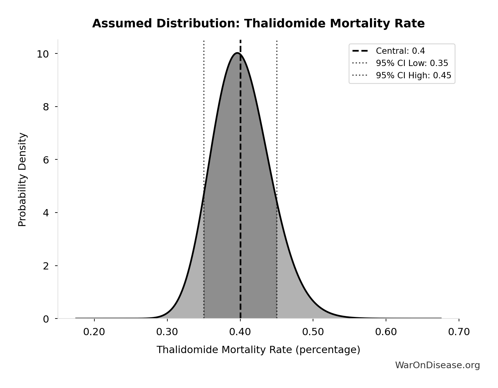
- Thalidomide Mortality Rate 📊: 40% (95% CI: 35% - 45%)
- Thalidomide US Cases Prevented 🔢: 900 cases
\[ \begin{gathered} Deaths_{thal} \\ = Rate_{thal,mort} \times N_{thal,US,prevent} \\ = 40\% \times 900 \\ = 360 \\[0.5em] \text{where } N_{thal,US,prevent} \\ = N_{thal,global} \times Pct_{US,1960} \\ = 15{,}000 \times 6\% \\ = 900 \end{gathered} \]
~ Medium confidence
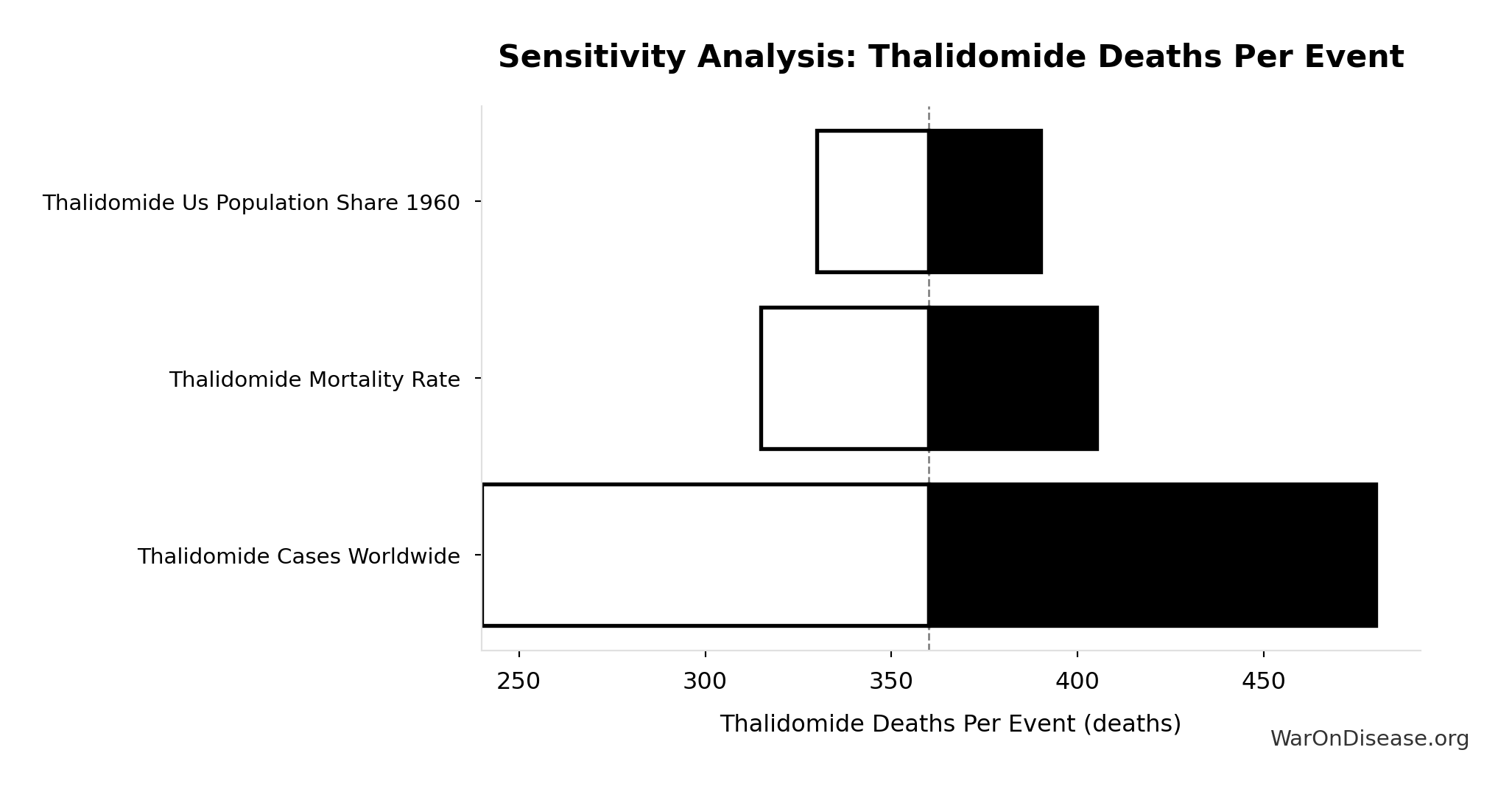
Sensitivity Analysis
Sensitivity Indices for Thalidomide Deaths Per Event
Regression-based sensitivity showing which inputs explain the most variance in the output.
| Input Parameter | Sensitivity Coefficient | Interpretation |
|---|---|---|
| Thalidomide US Cases Prevented | 1.5027 | Strong driver |
| Thalidomide Mortality Rate | -0.5048 | Strong driver |
Interpretation: Standardized coefficients show the change in output (in SD units) per 1 SD change in input. Values near ±1 indicate strong influence; values exceeding ±1 may occur with correlated inputs.
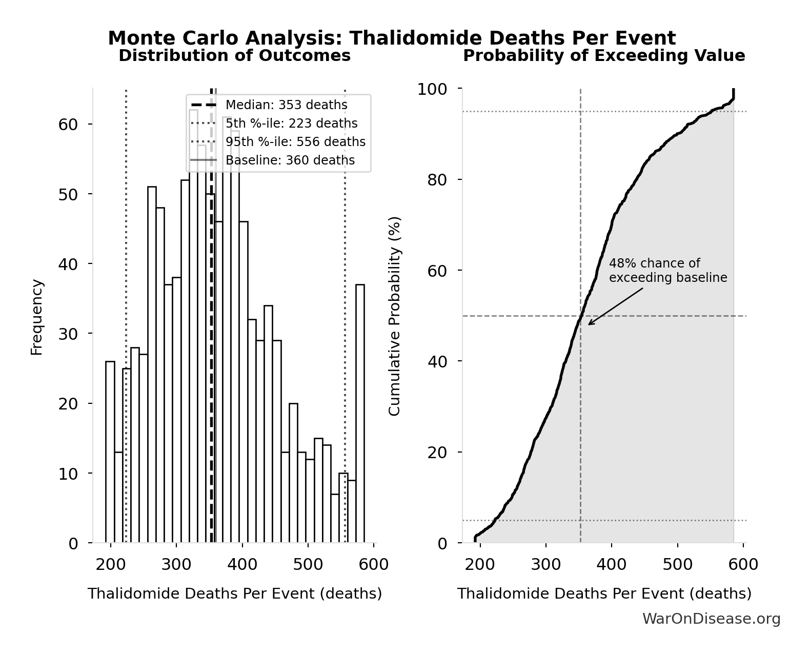
Monte Carlo Distribution
Simulation Results Summary: Thalidomide Deaths Per Event
| Statistic | Value |
|---|---|
| Baseline (deterministic) | 360 |
| Mean (expected value) | 364 |
| Median (50th percentile) | 353 |
| Standard Deviation | 95.8 |
| 90% Confidence Interval | [223, 556] |
The histogram shows the distribution of Thalidomide Deaths Per Event across 10,000 Monte Carlo simulations. The CDF (right) shows the probability of the outcome exceeding any given value, which is useful for risk assessment.
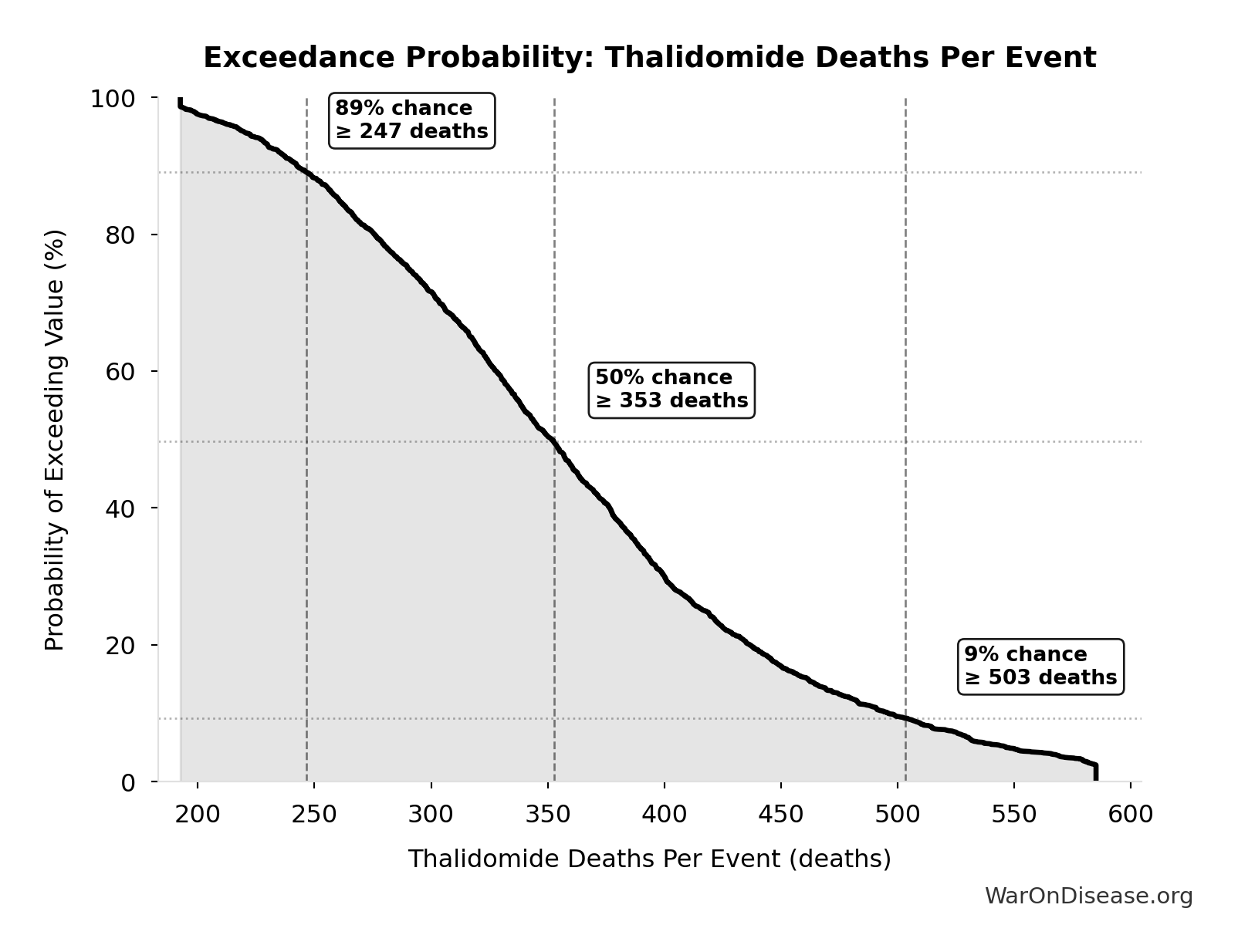
Exceedance Probability
This exceedance probability chart shows the likelihood that Thalidomide Deaths Per Event will exceed any given threshold. Higher curves indicate more favorable outcomes with greater certainty.
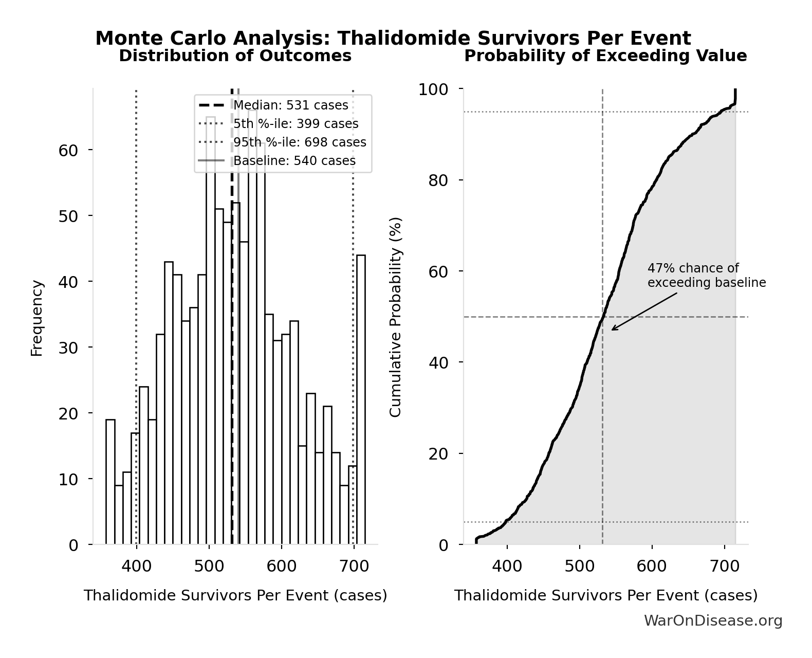
Thalidomide Survivors Per Event: 540 cases
Survivors per US-scale thalidomide event
Inputs:
- Thalidomide Mortality Rate 📊: 40% (95% CI: 35% - 45%)
- Thalidomide US Cases Prevented 🔢: 900 cases
\[ \begin{gathered} N_{thal,survive} \\ = N_{thal,US,prevent} \times (1 - Rate_{thal,mort}) \\ = 900 \times (1 - 40\%) \\ = 540 \\[0.5em] \text{where } N_{thal,US,prevent} \\ = N_{thal,global} \times Pct_{US,1960} \\ = 15{,}000 \times 6\% \\ = 900 \end{gathered} \]
~ Medium confidence
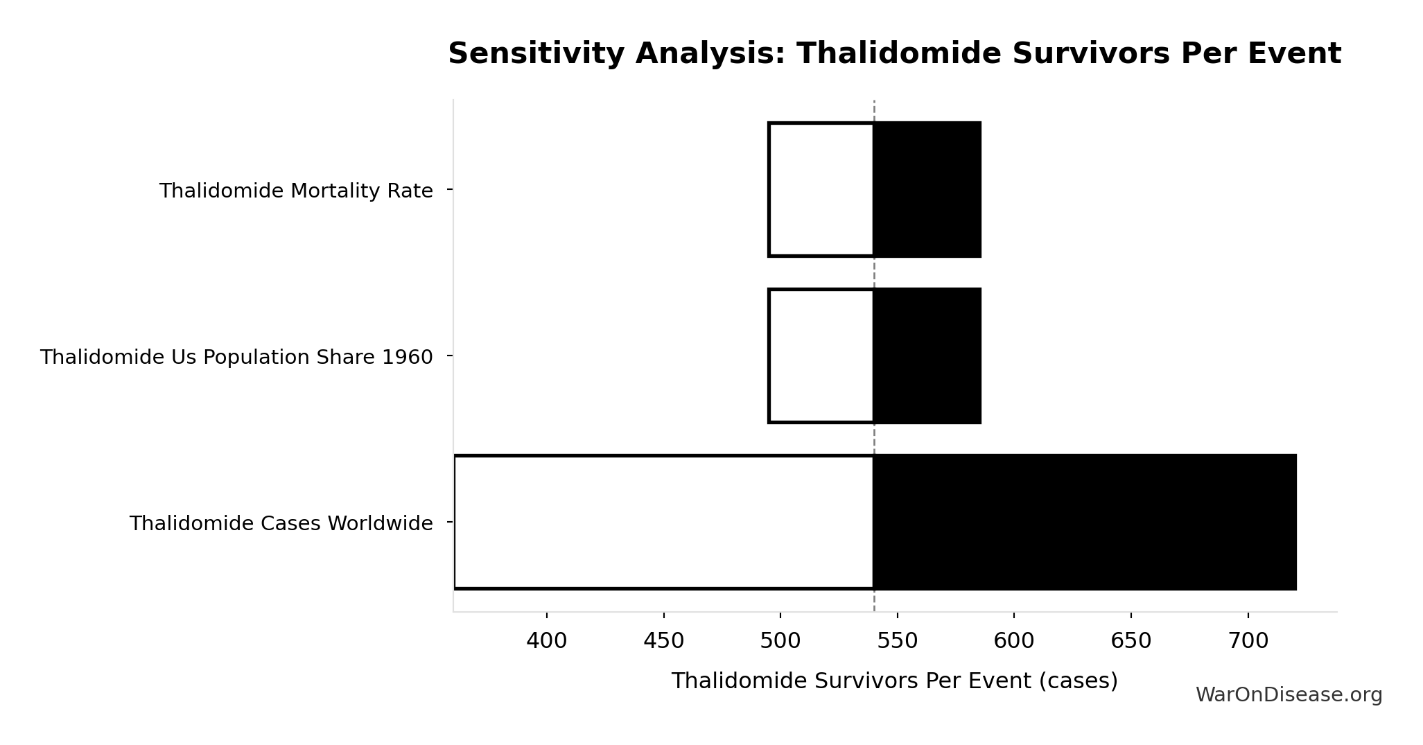
Sensitivity Analysis
Sensitivity Indices for Thalidomide Survivors Per Event
Regression-based sensitivity showing which inputs explain the most variance in the output.
| Input Parameter | Sensitivity Coefficient | Interpretation |
|---|---|---|
| Thalidomide Mortality Rate | 0.5607 | Strong driver |
| Thalidomide US Cases Prevented | 0.4398 | Moderate driver |
Interpretation: Standardized coefficients show the change in output (in SD units) per 1 SD change in input. Values near ±1 indicate strong influence; values exceeding ±1 may occur with correlated inputs.
Monte Carlo Distribution
Simulation Results Summary: Thalidomide Survivors Per Event
| Statistic | Value |
|---|---|
| Baseline (deterministic) | 540 |
| Mean (expected value) | 537 |
| Median (50th percentile) | 531 |
| Standard Deviation | 86.3 |
| 90% Confidence Interval | [399, 698] |
The histogram shows the distribution of Thalidomide Survivors Per Event across 10,000 Monte Carlo simulations. The CDF (right) shows the probability of the outcome exceeding any given value, which is useful for risk assessment.
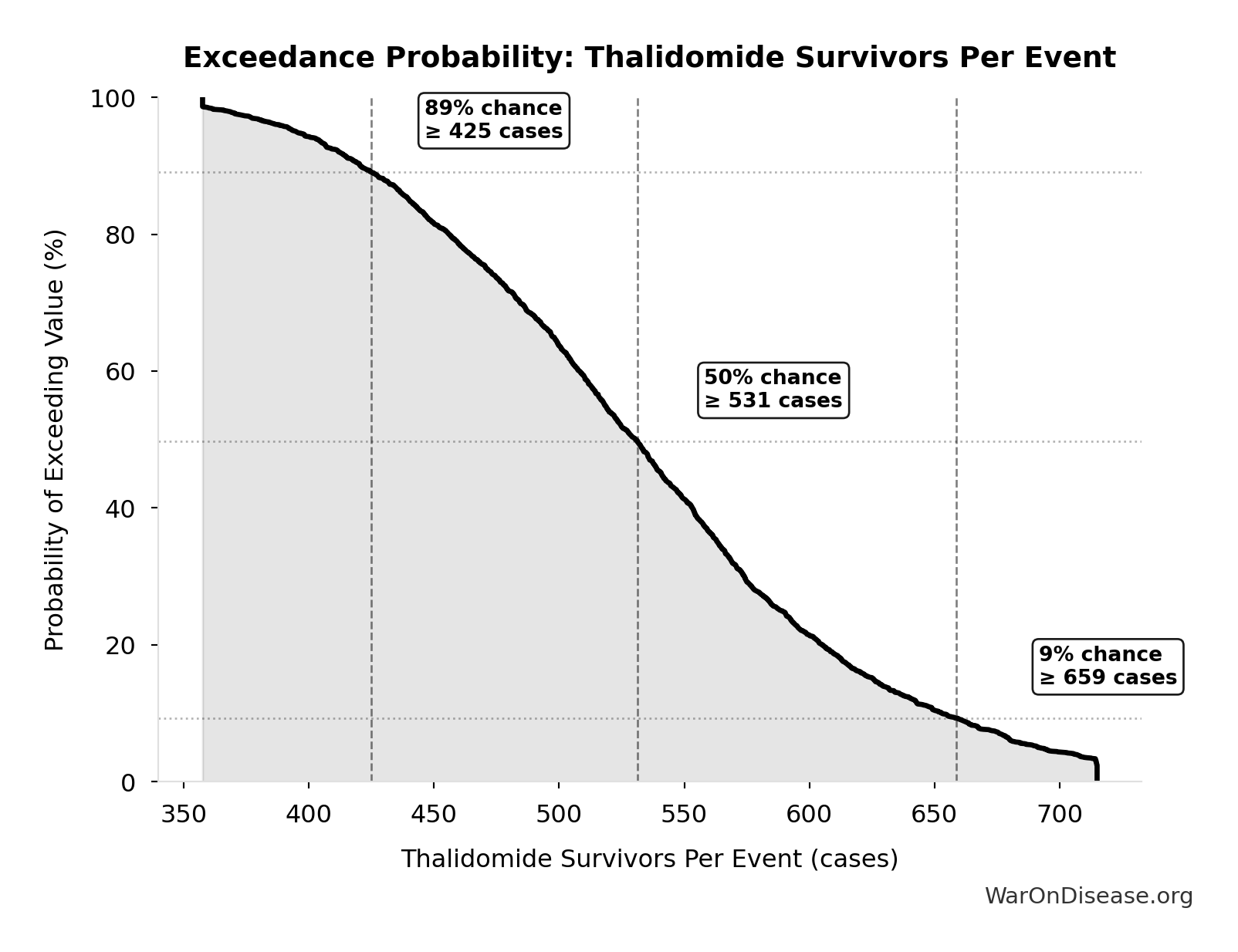
Exceedance Probability
This exceedance probability chart shows the likelihood that Thalidomide Survivors Per Event will exceed any given threshold. Higher curves indicate more favorable outcomes with greater certainty.
Thalidomide US Cases Prevented: 900 cases
Estimated US thalidomide cases prevented by FDA rejection
Inputs:
- Thalidomide Cases Worldwide 📊: 15.0k cases (95% CI: 10.0k cases - 20.0k cases)
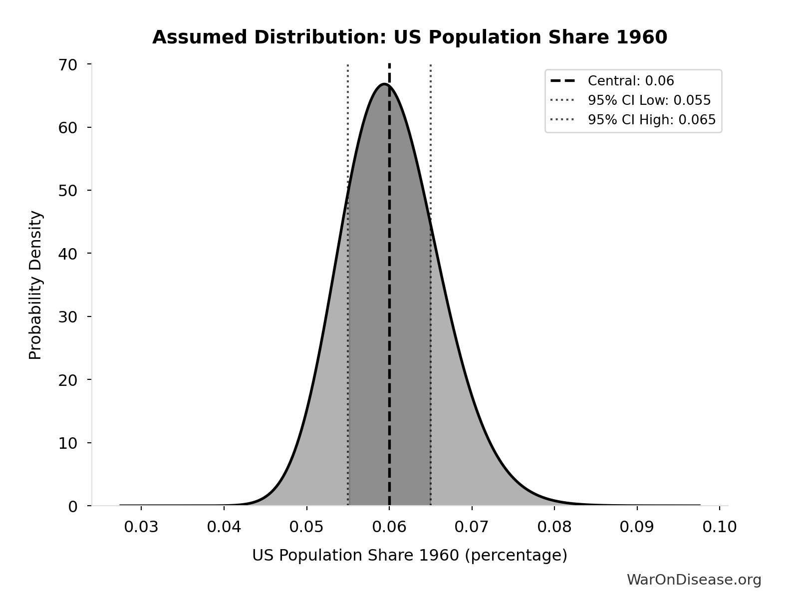
- US Population Share 1960 📊: 6% (95% CI: 5.5% - 6.5%)
\[ \begin{gathered} N_{thal,US,prevent} \\ = N_{thal,global} \times Pct_{US,1960} \\ = 15{,}000 \times 6\% \\ = 900 \end{gathered} \]
~ Medium confidence
Sensitivity Analysis
Sensitivity Indices for Thalidomide US Cases Prevented
Regression-based sensitivity showing which inputs explain the most variance in the output.
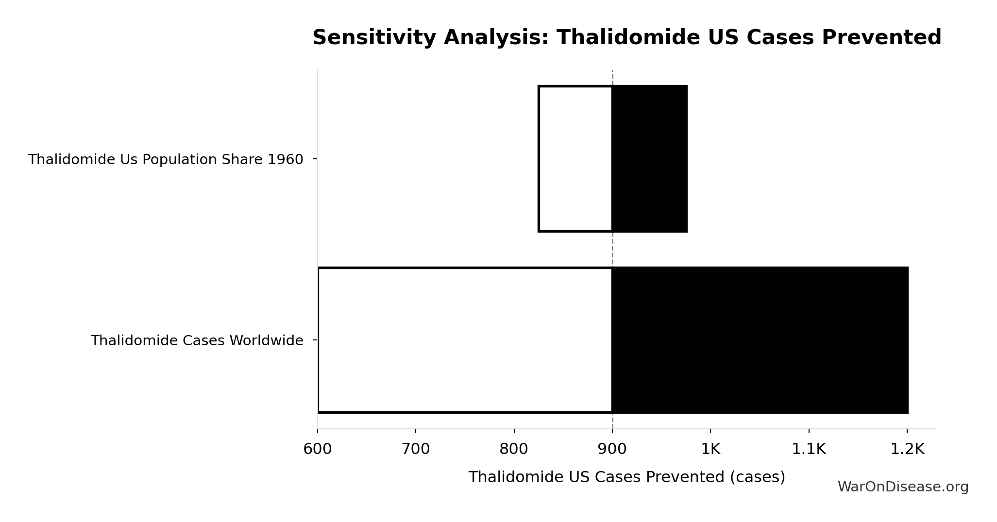
| Input Parameter | Sensitivity Coefficient | Interpretation |
|---|---|---|
| Thalidomide Cases Worldwide | 1.3746 | Strong driver |
| Thalidomide US Population Share 1960 | -0.3756 | Moderate driver |
Interpretation: Standardized coefficients show the change in output (in SD units) per 1 SD change in input. Values near ±1 indicate strong influence; values exceeding ±1 may occur with correlated inputs.
Monte Carlo Distribution
Simulation Results Summary: Thalidomide US Cases Prevented
| Statistic | Value |
|---|---|
| Baseline (deterministic) | 900 |
| Mean (expected value) | 901 |
| Median (50th percentile) | 884 |
| Standard Deviation | 182 |
| 90% Confidence Interval | [622, 1.25k] |
The histogram shows the distribution of Thalidomide US Cases Prevented across 10,000 Monte Carlo simulations. The CDF (right) shows the probability of the outcome exceeding any given value, which is useful for risk assessment.
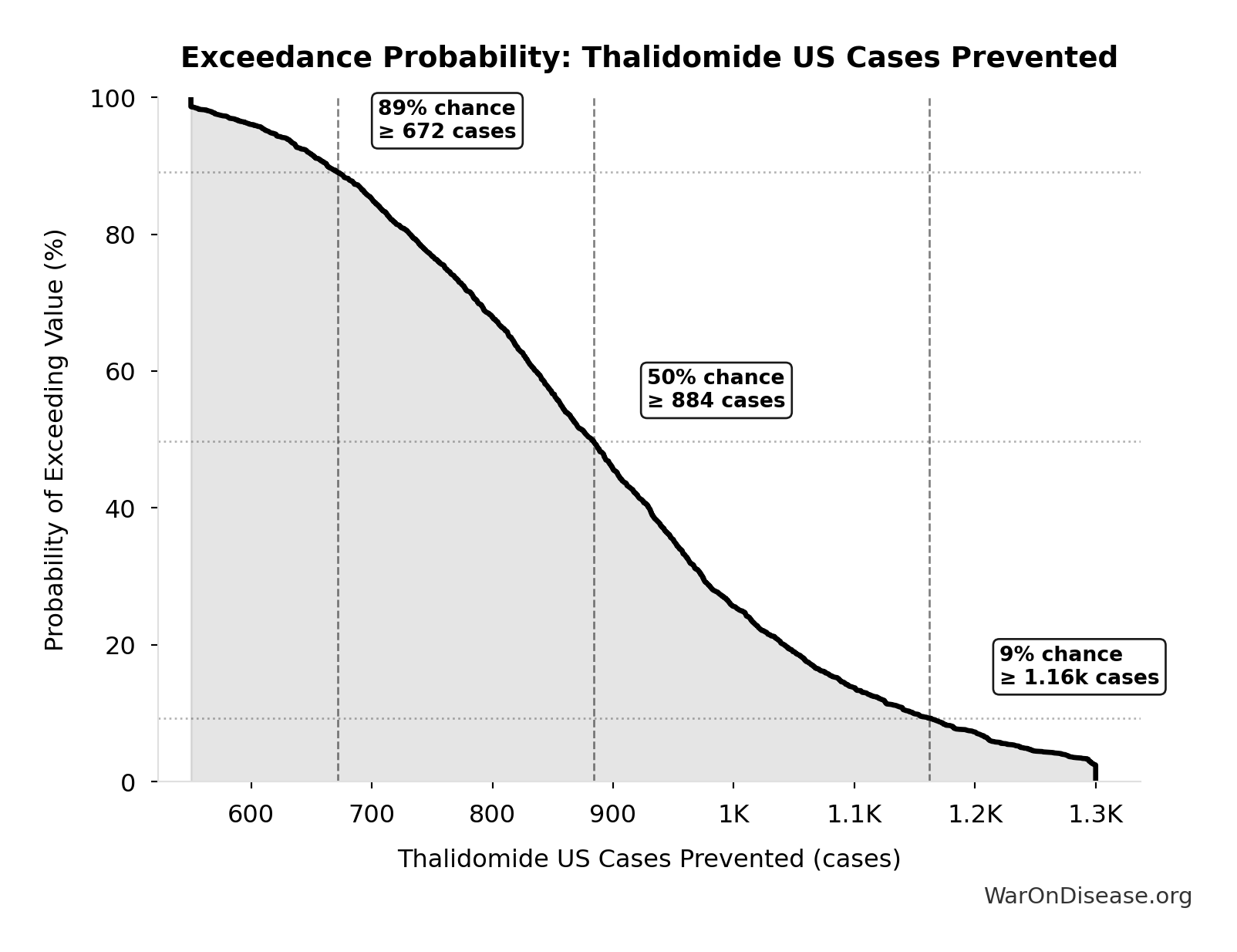
Exceedance Probability
This exceedance probability chart shows the likelihood that Thalidomide US Cases Prevented will exceed any given threshold. Higher curves indicate more favorable outcomes with greater certainty.
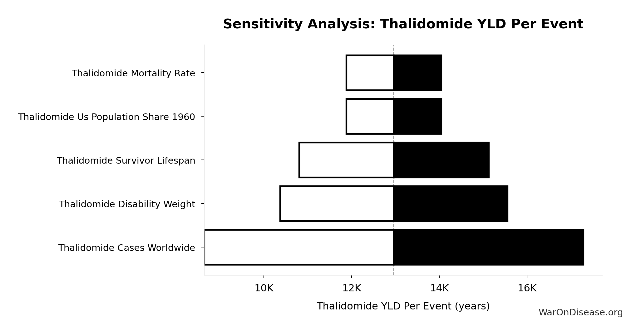
Thalidomide YLD Per Event: 13.0k years
Years Lived with Disability per thalidomide event
Inputs:
- Thalidomide Disability Weight 📊: 0.4:1 (95% CI: 0.32:1 - 0.48:1)
- Thalidomide Survivors Per Event 🔢: 540 cases
- Thalidomide Survivor Lifespan 📊: 60 years (95% CI: 50 years - 70 years)
\[ \begin{gathered} YLD_{thal} \\ = DW_{thal} \times N_{thal,survive} \times LE_{thal} \\ = 0.4 \times 540 \times 60 \\ = 13{,}000 \\[0.5em] \text{where } N_{thal,survive} \\ = N_{thal,US,prevent} \times (1 - Rate_{thal,mort}) \\ = 900 \times (1 - 40\%) \\ = 540 \\[0.5em] \text{where } N_{thal,US,prevent} \\ = N_{thal,global} \times Pct_{US,1960} \\ = 15{,}000 \times 6\% \\ = 900 \end{gathered} \]
~ Medium confidence
Sensitivity Analysis
Sensitivity Indices for Thalidomide YLD Per Event
Regression-based sensitivity showing which inputs explain the most variance in the output.
| Input Parameter | Sensitivity Coefficient | Interpretation |
|---|---|---|
| Thalidomide Disability Weight | 28.4785 | Strong driver |
| Thalidomide Survivor Lifespan | -23.4440 | Strong driver |
| Thalidomide Survivors Per Event | -4.0444 | Strong driver |
Interpretation: Standardized coefficients show the change in output (in SD units) per 1 SD change in input. Values near ±1 indicate strong influence; values exceeding ±1 may occur with correlated inputs.
Monte Carlo Distribution
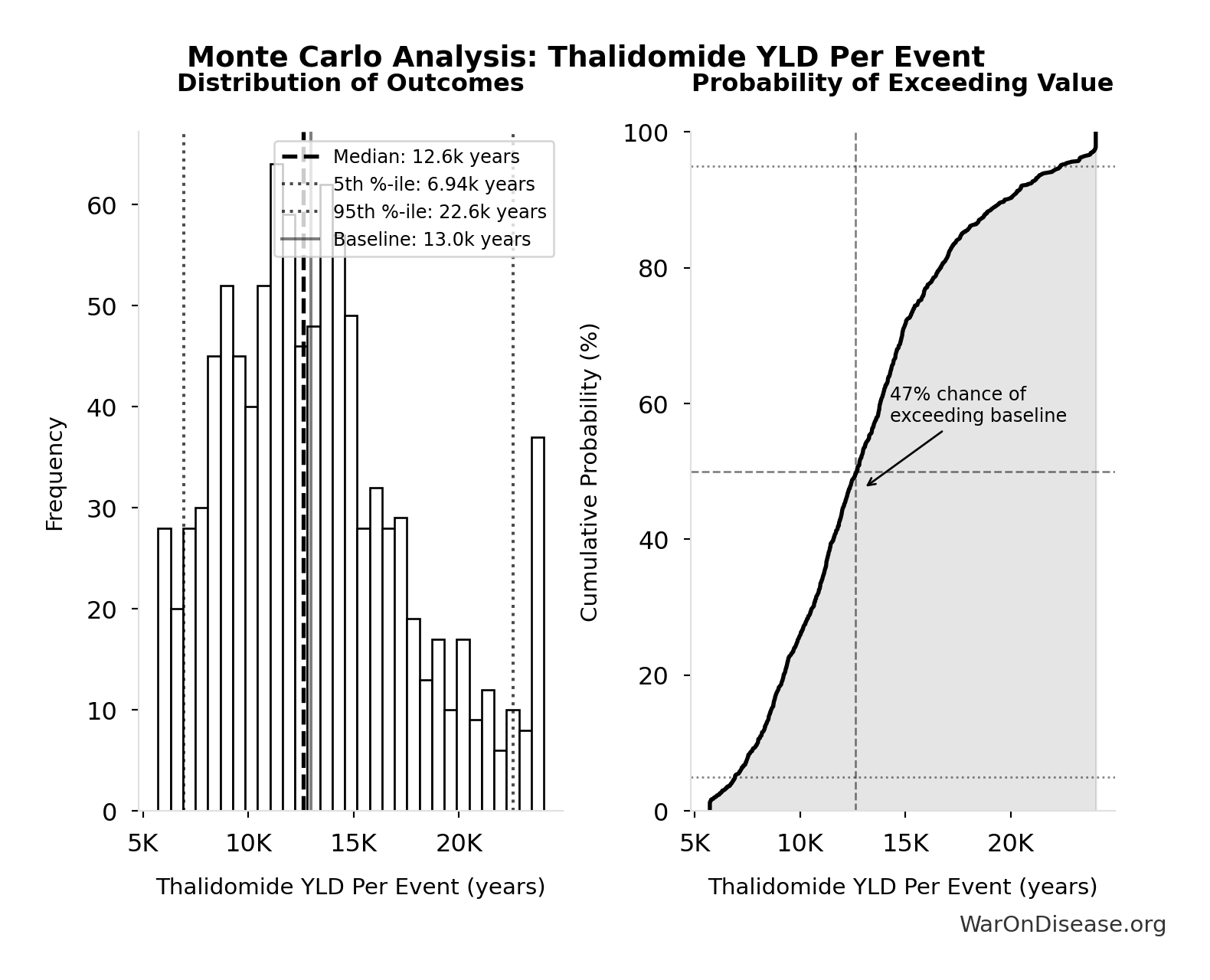
Simulation Results Summary: Thalidomide YLD Per Event
| Statistic | Value |
|---|---|
| Baseline (deterministic) | 13.0k |
| Mean (expected value) | 13.3k |
| Median (50th percentile) | 12.6k |
| Standard Deviation | 4.50k |
| 90% Confidence Interval | [6.94k, 22.6k] |
The histogram shows the distribution of Thalidomide YLD Per Event across 10,000 Monte Carlo simulations. The CDF (right) shows the probability of the outcome exceeding any given value, which is useful for risk assessment.
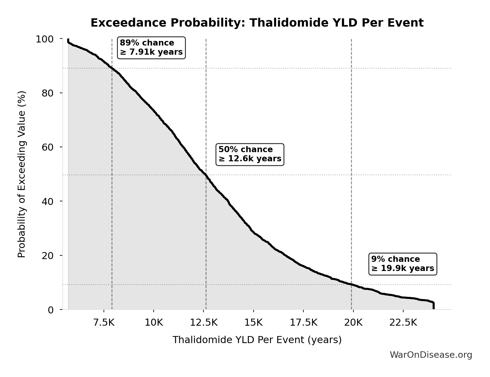
Exceedance Probability
This exceedance probability chart shows the likelihood that Thalidomide YLD Per Event will exceed any given threshold. Higher curves indicate more favorable outcomes with greater certainty.
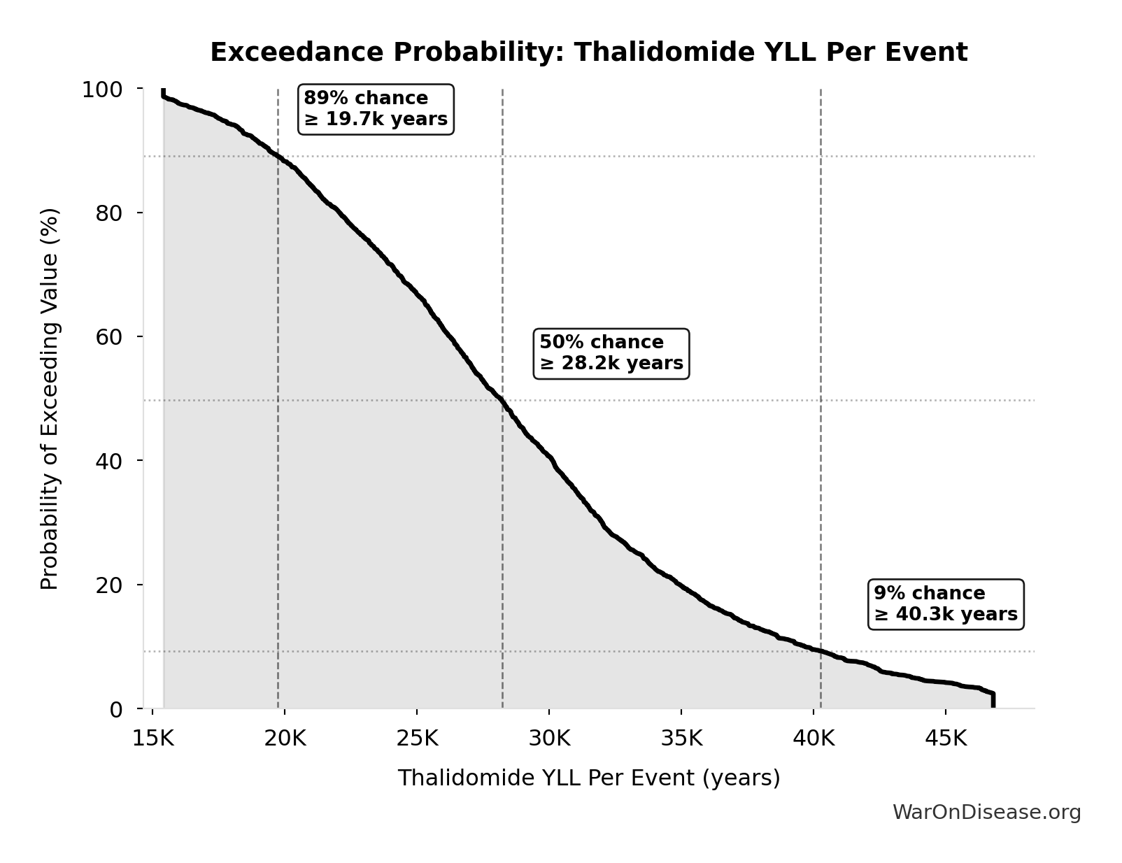
Thalidomide YLL Per Event: 28.8k years
Years of Life Lost per thalidomide event (infant deaths)
Inputs:
- Thalidomide Deaths Per Event 🔢: 360 deaths
\[ \begin{gathered} YLL_{thal} = Deaths_{thal} \times 80 = 360 \times 80 = 28{,}800 \\[0.5em] \text{where } Deaths_{thal} \\ = Rate_{thal,mort} \times N_{thal,US,prevent} \\ = 40\% \times 900 \\ = 360 \\[0.5em] \text{where } N_{thal,US,prevent} \\ = N_{thal,global} \times Pct_{US,1960} \\ = 15{,}000 \times 6\% \\ = 900 \end{gathered} \]
~ Medium confidence
Sensitivity Analysis
Sensitivity Indices for Thalidomide YLL Per Event
Regression-based sensitivity showing which inputs explain the most variance in the output.
| Input Parameter | Sensitivity Coefficient | Interpretation |
|---|---|---|
| Thalidomide Deaths Per Event | 1.0000 | Strong driver |
Interpretation: Standardized coefficients show the change in output (in SD units) per 1 SD change in input. Values near ±1 indicate strong influence; values exceeding ±1 may occur with correlated inputs.
Monte Carlo Distribution
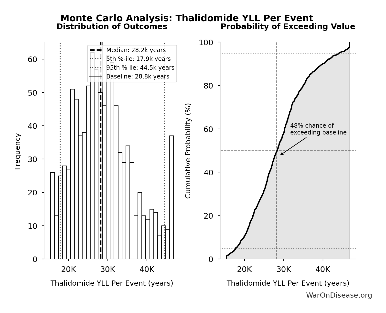
Simulation Results Summary: Thalidomide YLL Per Event
| Statistic | Value |
|---|---|
| Baseline (deterministic) | 28.8k |
| Mean (expected value) | 29.2k |
| Median (50th percentile) | 28.2k |
| Standard Deviation | 7.67k |
| 90% Confidence Interval | [17.9k, 44.5k] |
The histogram shows the distribution of Thalidomide YLL Per Event across 10,000 Monte Carlo simulations. The CDF (right) shows the probability of the outcome exceeding any given value, which is useful for risk assessment.
Exceedance Probability
This exceedance probability chart shows the likelihood that Thalidomide YLL Per Event will exceed any given threshold. Higher curves indicate more favorable outcomes with greater certainty.
Ratio of Type Ii Error Cost to Type I Error Benefit: 3.07k:1
Ratio of Type II error cost to Type I error benefit (harm from delay vs. harm prevented)
Inputs:
- Total DALYs Lost from Disease Eradication Delay 🔢: 7.94B DALYs
- Maximum DALYs Saved by FDA Preventing Unsafe Drugs (1962-2024) 🔢: 2.59M DALYs
\[ \begin{gathered} Ratio_{TypeII} = \frac{DALYs_{lag}}{DALY_{TypeI}} = \frac{7.94B}{2.59M} = 3{,}070 \\[0.5em] \text{where } DALYs_{lag} = YLL_{lag} + YLD_{lag} = 7.07B + 873M = 7.94B \\[0.5em] \text{where } YLL_{lag} \\ = Deaths_{lag} \times (LE_{global} - Age_{death,delay}) \\ = 416M \times (79 - 62) \\ = 7.07B \\[0.5em] \text{where } Deaths_{lag} \\ = T_{lag} \times Deaths_{disease,daily} \times 338 \\ = 8.2 \times 150{,}000 \times 338 \\ = 416M \\[0.5em] \text{where } YLD_{lag} \\ = Deaths_{lag} \times T_{suffering} \times DW_{chronic} \\ = 416M \times 6 \times 0.35 \\ = 873M \\[0.5em] \text{where } Deaths_{lag} \\ = T_{lag} \times Deaths_{disease,daily} \times 338 \\ = 8.2 \times 150{,}000 \times 338 \\ = 416M \\[0.5em] \text{where } DALY_{TypeI} = DALY_{thal} \times 62 = 41{,}800 \times 62 = 2.59M \\[0.5em] \text{where } DALY_{thal} \\ = YLD_{thal} + YLL_{thal} \\ = 13{,}000 + 28{,}800 \\ = 41{,}800 \\[0.5em] \text{where } YLD_{thal} \\ = DW_{thal} \times N_{thal,survive} \times LE_{thal} \\ = 0.4 \times 540 \times 60 \\ = 13{,}000 \\[0.5em] \text{where } N_{thal,survive} \\ = N_{thal,US,prevent} \times (1 - Rate_{thal,mort}) \\ = 900 \times (1 - 40\%) \\ = 540 \\[0.5em] \text{where } N_{thal,US,prevent} \\ = N_{thal,global} \times Pct_{US,1960} \\ = 15{,}000 \times 6\% \\ = 900 \\[0.5em] \text{where } YLL_{thal} = Deaths_{thal} \times 80 = 360 \times 80 = 28{,}800 \\[0.5em] \text{where } Deaths_{thal} \\ = Rate_{thal,mort} \times N_{thal,US,prevent} \\ = 40\% \times 900 \\ = 360 \\[0.5em] \text{where } N_{thal,US,prevent} \\ = N_{thal,global} \times Pct_{US,1960} \\ = 15{,}000 \times 6\% \\ = 900 \end{gathered} \]
Methodology: ../appendix/invisible-graveyard#risk-analysis
~ Medium confidence
Sensitivity Analysis
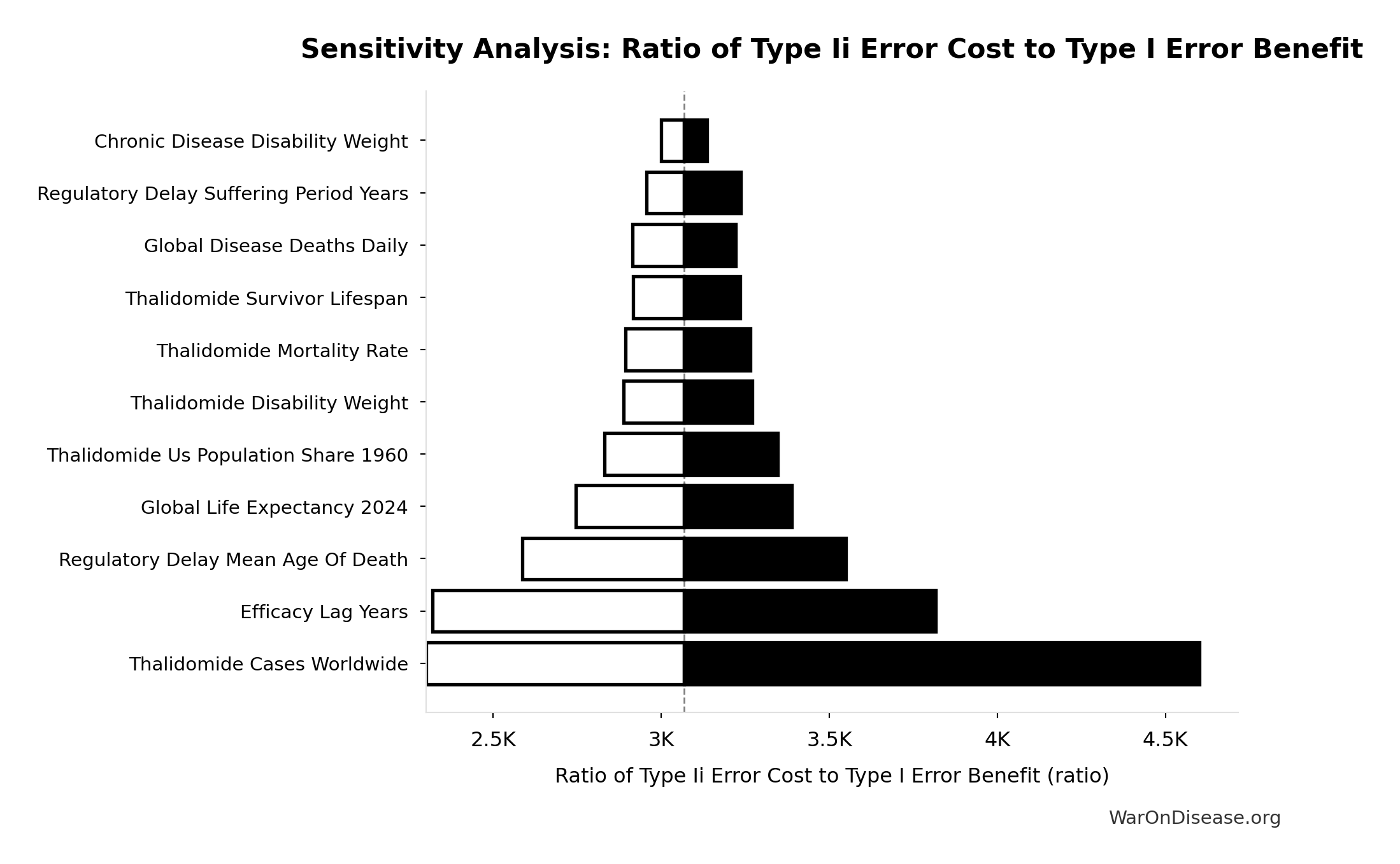
Sensitivity Indices for Ratio of Type Ii Error Cost to Type I Error Benefit
Regression-based sensitivity showing which inputs explain the most variance in the output.
| Input Parameter | Sensitivity Coefficient | Interpretation |
|---|---|---|
| dFDA Efficacy Lag Elimination DALYs | 7.2872 | Strong driver |
| Type I Error Benefit DALYs | -7.1207 | Strong driver |
Interpretation: Standardized coefficients show the change in output (in SD units) per 1 SD change in input. Values near ±1 indicate strong influence; values exceeding ±1 may occur with correlated inputs.
Monte Carlo Distribution
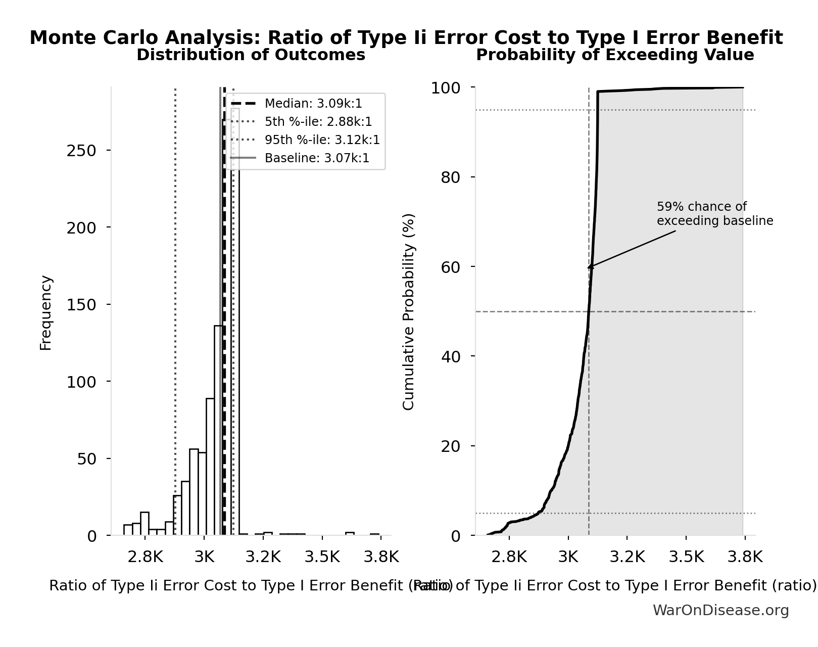
Simulation Results Summary: Ratio of Type Ii Error Cost to Type I Error Benefit
| Statistic | Value |
|---|---|
| Baseline (deterministic) | 3.07k:1 |
| Mean (expected value) | 3.05k:1 |
| Median (50th percentile) | 3.09k:1 |
| Standard Deviation | 101:1 |
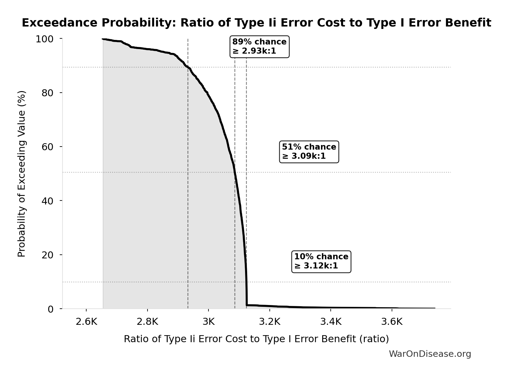
| 90% Confidence Interval | [2.88k:1, 3.12k:1] |
The histogram shows the distribution of Ratio of Type Ii Error Cost to Type I Error Benefit across 10,000 Monte Carlo simulations. The CDF (right) shows the probability of the outcome exceeding any given value, which is useful for risk assessment.
Exceedance Probability
This exceedance probability chart shows the likelihood that Ratio of Type Ii Error Cost to Type I Error Benefit will exceed any given threshold. Higher curves indicate more favorable outcomes with greater certainty.
Maximum DALYs Saved by FDA Preventing Unsafe Drugs (1962-2024): 2.59M DALYs
Maximum DALYs saved by FDA preventing unsafe drugs over 62-year period 1962-2024 (extreme overestimate: one Thalidomide-scale event per year)
Inputs:
- Thalidomide DALYs Per Event 🔢: 41.8k DALYs
\[ \begin{gathered} DALY_{TypeI} = DALY_{thal} \times 62 = 41{,}800 \times 62 = 2.59M \\[0.5em] \text{where } DALY_{thal} \\ = YLD_{thal} + YLL_{thal} \\ = 13{,}000 + 28{,}800 \\ = 41{,}800 \\[0.5em] \text{where } YLD_{thal} \\ = DW_{thal} \times N_{thal,survive} \times LE_{thal} \\ = 0.4 \times 540 \times 60 \\ = 13{,}000 \\[0.5em] \text{where } N_{thal,survive} \\ = N_{thal,US,prevent} \times (1 - Rate_{thal,mort}) \\ = 900 \times (1 - 40\%) \\ = 540 \\[0.5em] \text{where } N_{thal,US,prevent} \\ = N_{thal,global} \times Pct_{US,1960} \\ = 15{,}000 \times 6\% \\ = 900 \\[0.5em] \text{where } YLL_{thal} = Deaths_{thal} \times 80 = 360 \times 80 = 28{,}800 \\[0.5em] \text{where } Deaths_{thal} \\ = Rate_{thal,mort} \times N_{thal,US,prevent} \\ = 40\% \times 900 \\ = 360 \\[0.5em] \text{where } N_{thal,US,prevent} \\ = N_{thal,global} \times Pct_{US,1960} \\ = 15{,}000 \times 6\% \\ = 900 \end{gathered} \]
Methodology: ../appendix/invisible-graveyard#risk-analysis
? Low confidence
Sensitivity Analysis
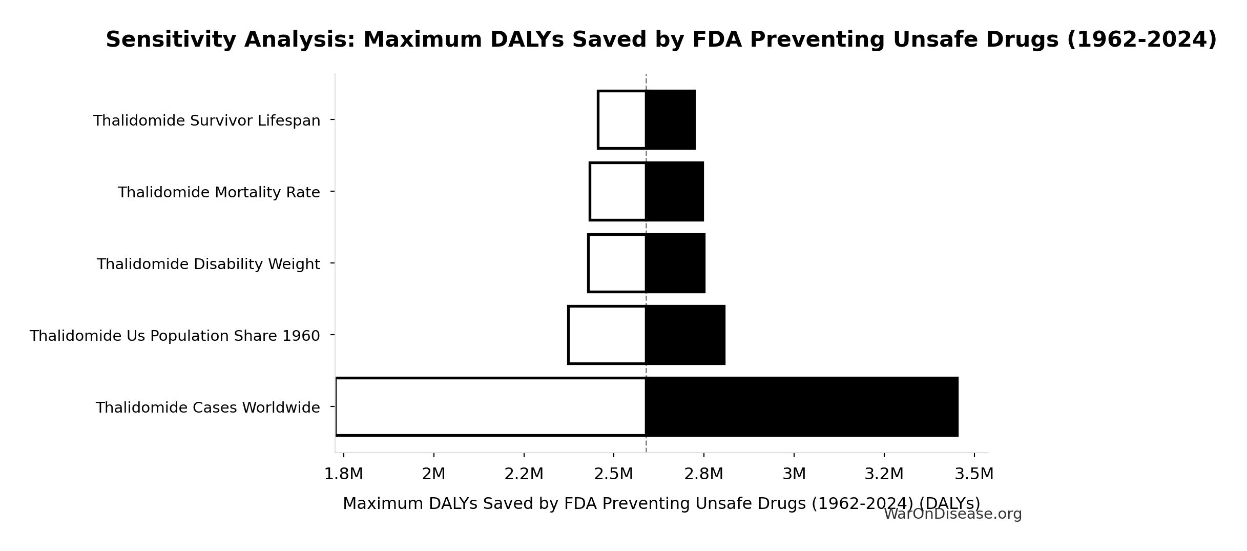
Sensitivity Indices for Maximum DALYs Saved by FDA Preventing Unsafe Drugs (1962-2024)
Regression-based sensitivity showing which inputs explain the most variance in the output.
| Input Parameter | Sensitivity Coefficient | Interpretation |
|---|---|---|
| Thalidomide DALYs Per Event | 1.0000 | Strong driver |
Interpretation: Standardized coefficients show the change in output (in SD units) per 1 SD change in input. Values near ±1 indicate strong influence; values exceeding ±1 may occur with correlated inputs.
Monte Carlo Distribution
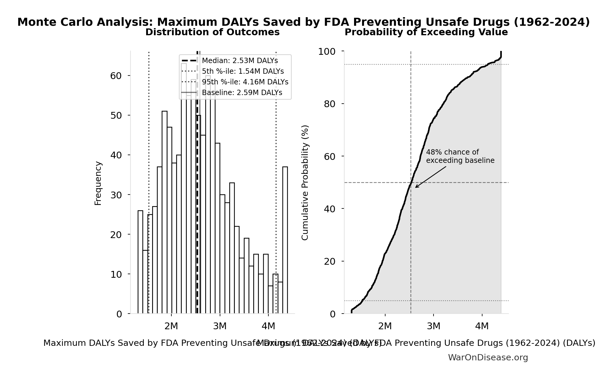
Simulation Results Summary: Maximum DALYs Saved by FDA Preventing Unsafe Drugs (1962-2024)
| Statistic | Value |
|---|---|
| Baseline (deterministic) | 2.59M |
| Mean (expected value) | 2.63M |
| Median (50th percentile) | 2.53M |
| Standard Deviation | 754k |
| 90% Confidence Interval | [1.54M, 4.16M] |
The histogram shows the distribution of Maximum DALYs Saved by FDA Preventing Unsafe Drugs (1962-2024) across 10,000 Monte Carlo simulations. The CDF (right) shows the probability of the outcome exceeding any given value, which is useful for risk assessment.
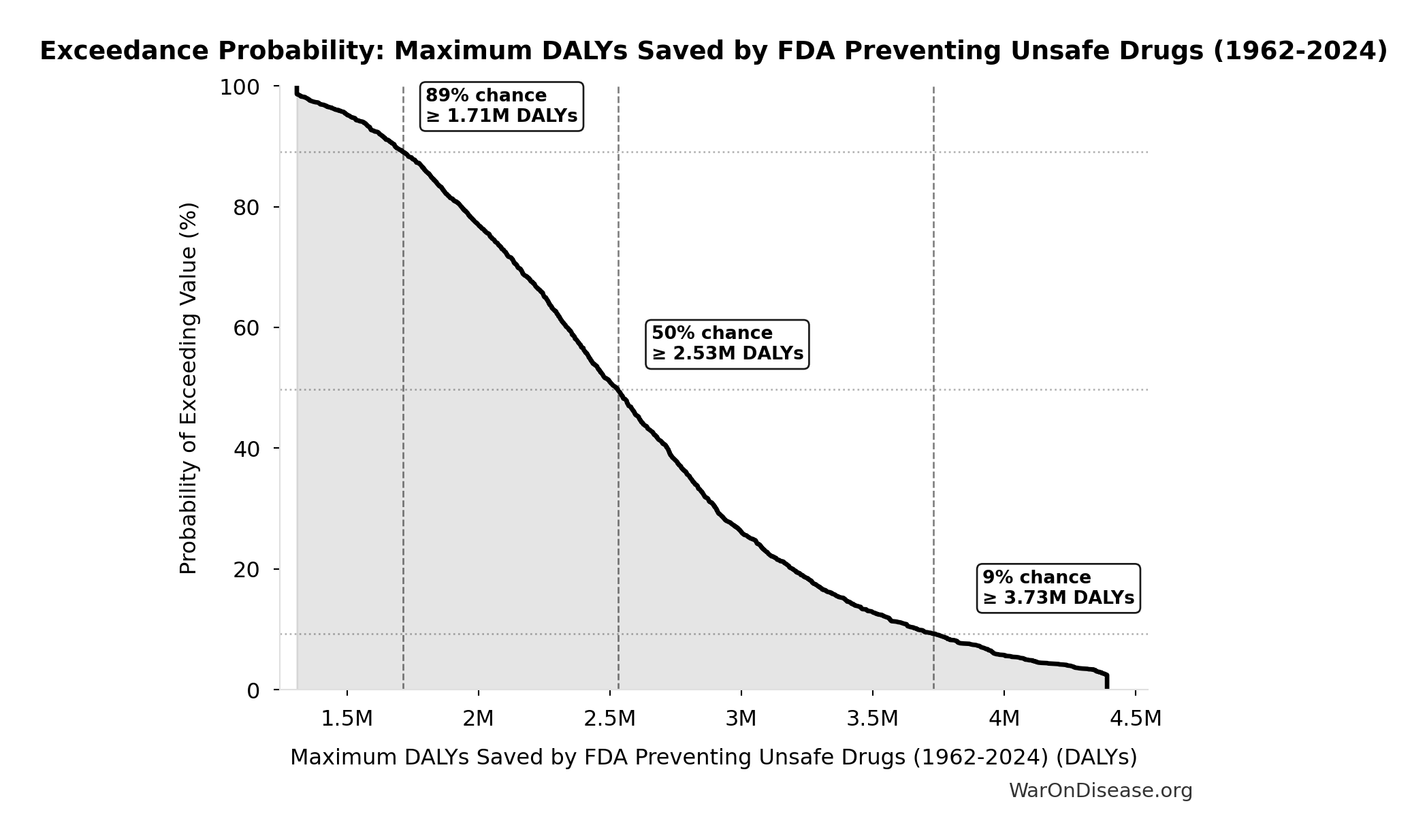
Exceedance Probability
This exceedance probability chart shows the likelihood that Maximum DALYs Saved by FDA Preventing Unsafe Drugs (1962-2024) will exceed any given threshold. Higher curves indicate more favorable outcomes with greater certainty.
External Data Sources
Parameters sourced from peer-reviewed publications, institutional databases, and authoritative reports.
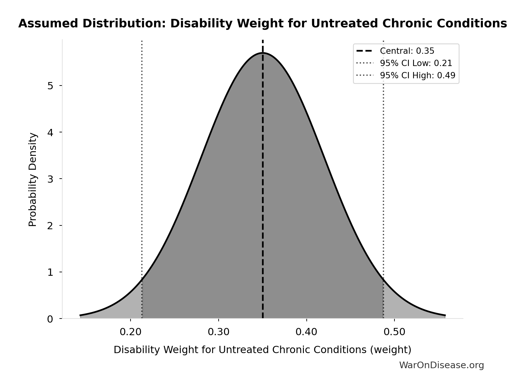
Disability Weight for Untreated Chronic Conditions: 0.35 weight
Disability weight for untreated chronic conditions (WHO Global Burden of Disease)
Source:18
Uncertainty Range
Technical: Distribution: Normal (SE: 0.07 weight)
Input Distribution
This chart shows the assumed probability distribution for this parameter. The shaded region represents the 95% confidence interval where we expect the true value to fall.
~ Medium confidence • 📊 Peer-reviewed
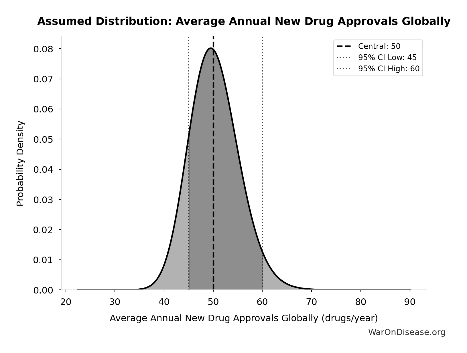
Average Annual New Drug Approvals Globally: 50 drugs/year
Average annual new drug approvals globally
Source:29
Uncertainty Range
Technical: 95% CI: [45 drugs/year, 60 drugs/year] • Distribution: Lognormal
What this means: This estimate has moderate uncertainty. The true value likely falls between 45 drugs/year and 60 drugs/year (±15%). This represents a reasonable range that our Monte Carlo simulations account for when calculating overall uncertainty in the results.
The lognormal distribution means values can’t go negative and have a longer tail toward higher values (common for costs and populations).
Input Distribution
This chart shows the assumed probability distribution for this parameter. The shaded region represents the 95% confidence interval where we expect the true value to fall.
✓ High confidence
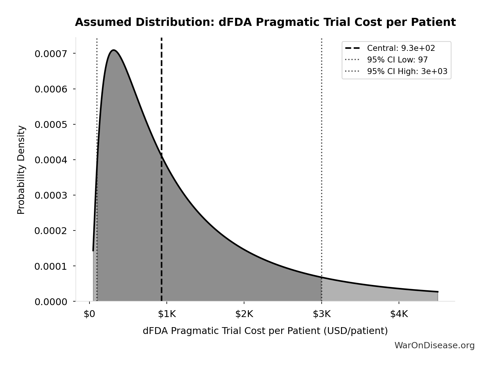
dFDA Pragmatic Trial Cost per Patient: $929
dFDA pragmatic trial cost per patient. Uses ADAPTABLE trial ($929) as DELIBERATELY CONSERVATIVE central estimate. Harvard meta-analysis of 108 trials found median of only $97/patient - our estimate may overstate costs by 10x. Confidence interval spans meta-analysis median to complex chronic disease trials.
Source:1
Uncertainty Range
Technical: 95% CI: [$97, $3K] • Distribution: Lognormal
What this means: This estimate is highly uncertain. The true value likely falls between $97 and $3K (±156%). This represents a very wide range that our Monte Carlo simulations account for when calculating overall uncertainty in the results.
The lognormal distribution means values can’t go negative and have a longer tail toward higher values (common for costs and populations).
Input Distribution
This chart shows the assumed probability distribution for this parameter. The shaded region represents the 95% confidence interval where we expect the true value to fall.
~ Medium confidence
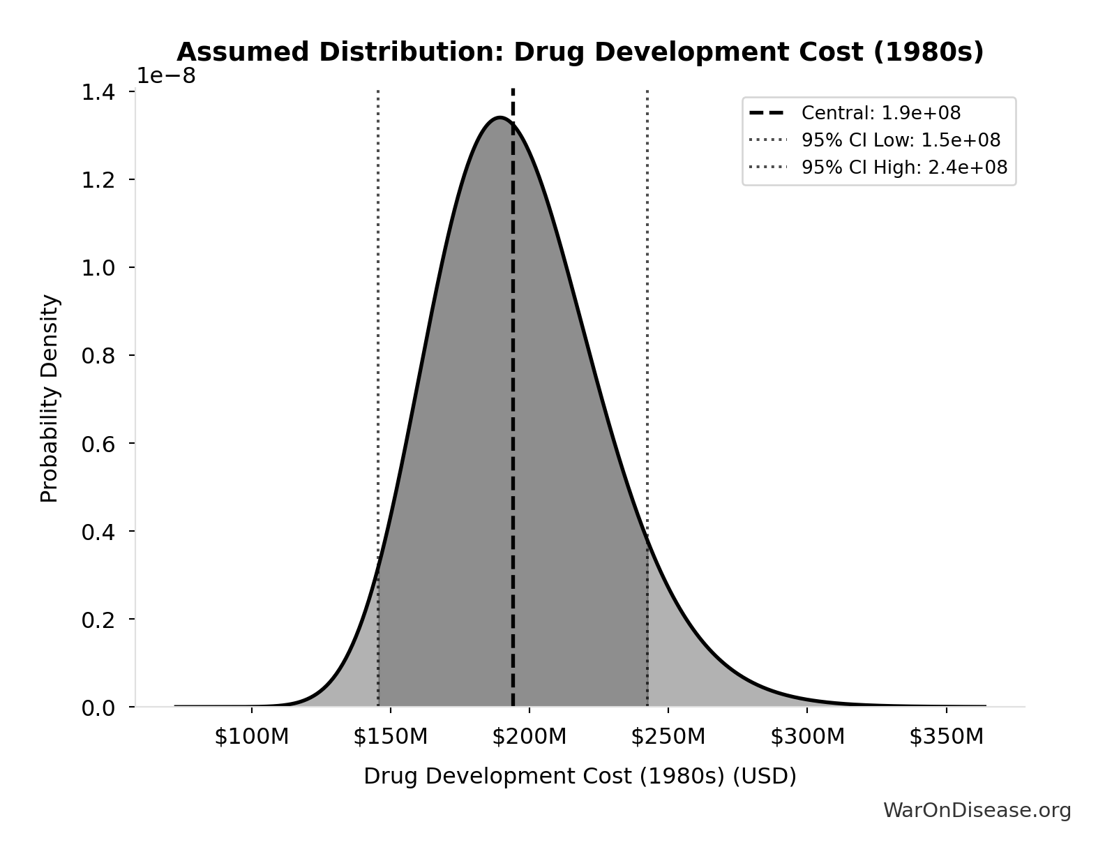
Drug Development Cost (1980s): $194M
Drug development cost in 1980s (compounded to approval, 1990 dollars)
Source:35
Uncertainty Range
Technical: 95% CI: [$146M, $242M] • Distribution: Lognormal
What this means: This estimate has moderate uncertainty. The true value likely falls between $146M and $242M (±25%). This represents a reasonable range that our Monte Carlo simulations account for when calculating overall uncertainty in the results.
The lognormal distribution means values can’t go negative and have a longer tail toward higher values (common for costs and populations).
Input Distribution
This chart shows the assumed probability distribution for this parameter. The shaded region represents the 95% confidence interval where we expect the true value to fall.
✓ High confidence
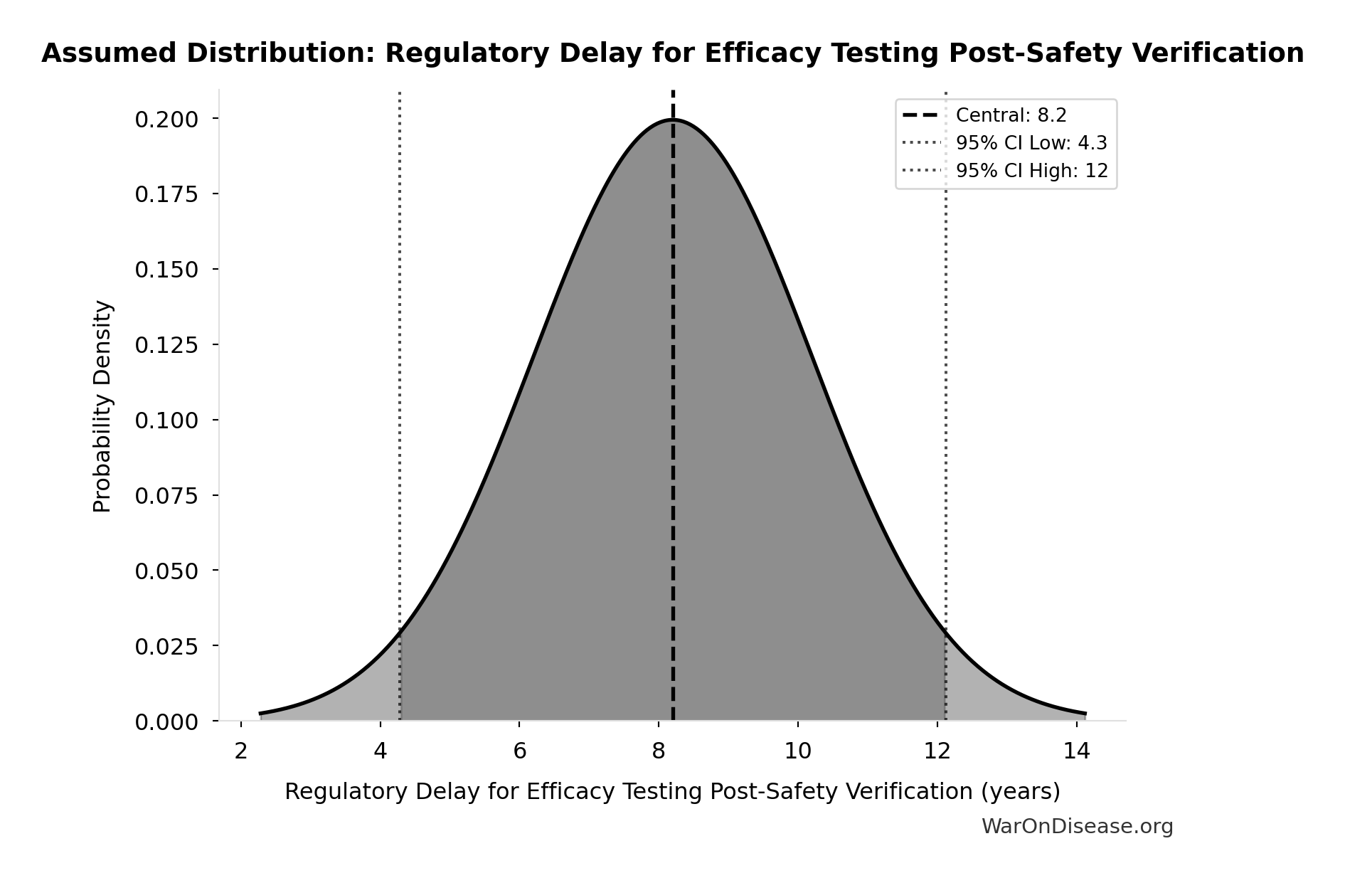
Regulatory Delay for Efficacy Testing Post-Safety Verification: 8.2 years
Regulatory delay for efficacy testing (Phase II/III) post-safety verification. Based on BIO 2021 industry survey. Note: This is for drugs that COMPLETE the pipeline - survivor bias means actual delay for any given disease may be longer if candidates fail and must restart.
Source:41
Uncertainty Range
Technical: Distribution: Normal (SE: 2 years)
Input Distribution
This chart shows the assumed probability distribution for this parameter. The shaded region represents the 95% confidence interval where we expect the true value to fall.
~ Medium confidence • 📊 Peer-reviewed • Updated 2021
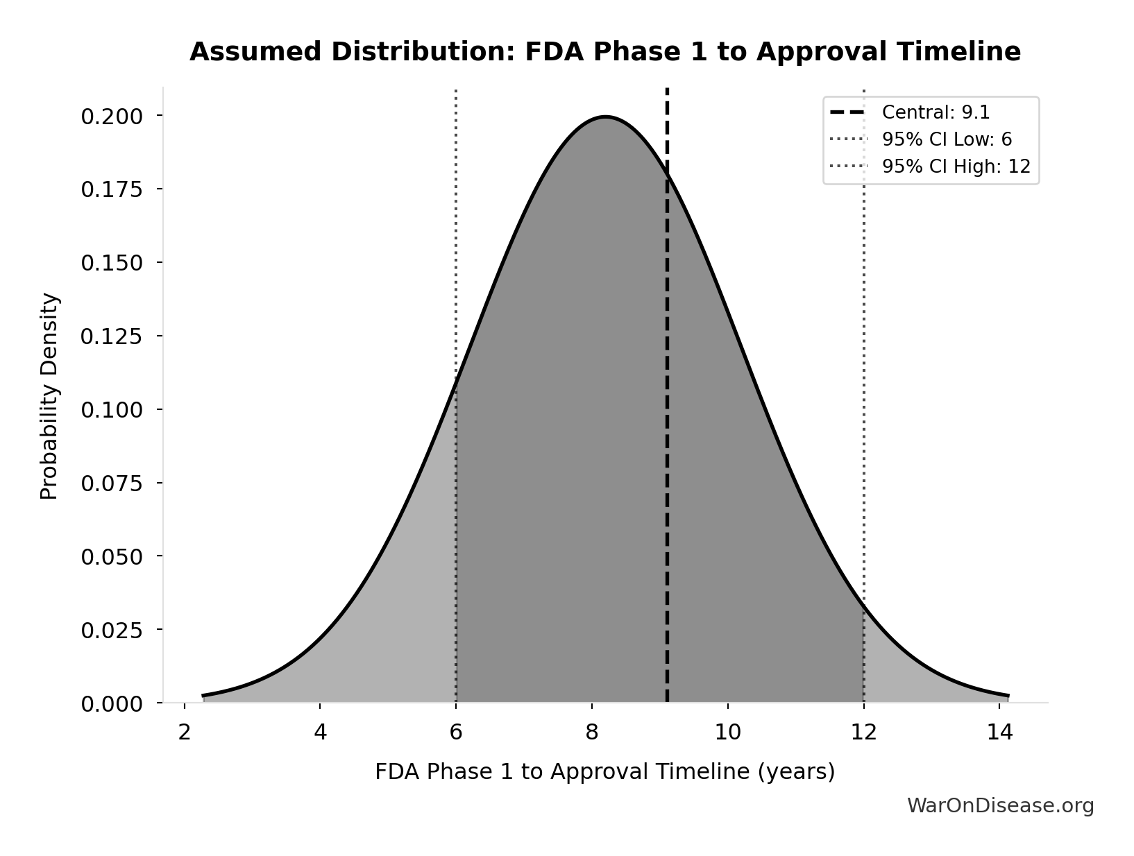
FDA Phase 1 to Approval Timeline: 9.1 years
FDA timeline from Phase 1 start to approval (Phase 1-3 + NDA review)
Source:44
Uncertainty Range
Technical: 95% CI: [6 years, 12 years] • Distribution: Gamma (SE: 2 years)
What this means: There’s significant uncertainty here. The true value likely falls between 6 years and 12 years (±33%). This represents a wide range that our Monte Carlo simulations account for when calculating overall uncertainty in the results.
The gamma distribution means values follow a specific statistical pattern.
Input Distribution
This chart shows the assumed probability distribution for this parameter. The shaded region represents the 95% confidence interval where we expect the true value to fall.
✓ High confidence
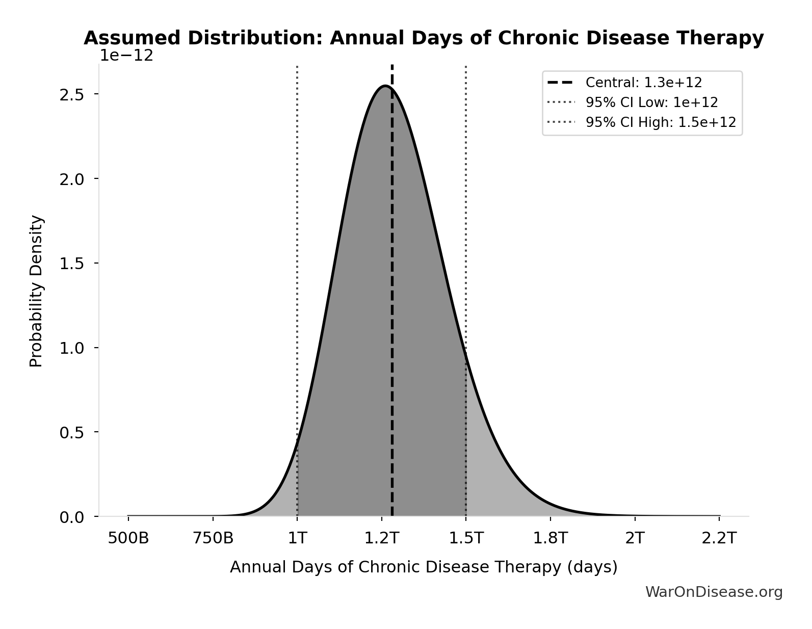
Annual Days of Chronic Disease Therapy: 1.28T days
Annual days of therapy for chronic conditions globally (diabetes, CVD, respiratory, cancer). IQVIA reports 1.8 trillion total days of therapy in 2019, with 71% for chronic conditions.
Source:57
Uncertainty Range
Technical: 95% CI: [1.00T days, 1.50T days] • Distribution: Lognormal
What this means: This estimate has moderate uncertainty. The true value likely falls between 1.00T days and 1.50T days (±20%). This represents a reasonable range that our Monte Carlo simulations account for when calculating overall uncertainty in the results.
The lognormal distribution means values can’t go negative and have a longer tail toward higher values (common for costs and populations).
Input Distribution
This chart shows the assumed probability distribution for this parameter. The shaded region represents the 95% confidence interval where we expect the true value to fall.
~ Medium confidence
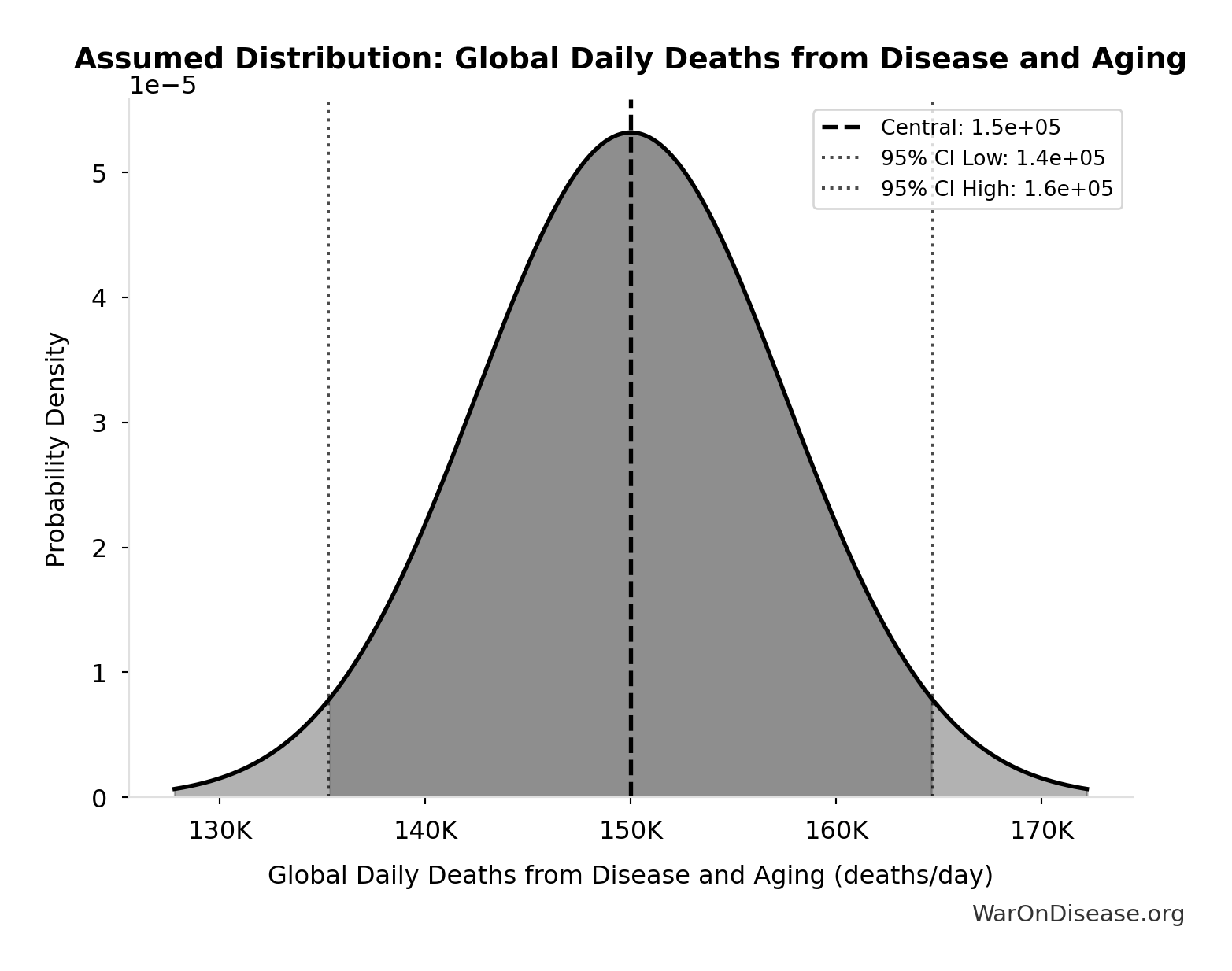
Global Daily Deaths from Disease and Aging: 150k deaths/day
Total global deaths per day from all disease and aging (WHO Global Burden of Disease 2024)
Source:18
Uncertainty Range
Technical: Distribution: Normal (SE: 7.50k deaths/day)
Input Distribution
This chart shows the assumed probability distribution for this parameter. The shaded region represents the 95% confidence interval where we expect the true value to fall.
✓ High confidence • 📊 Peer-reviewed
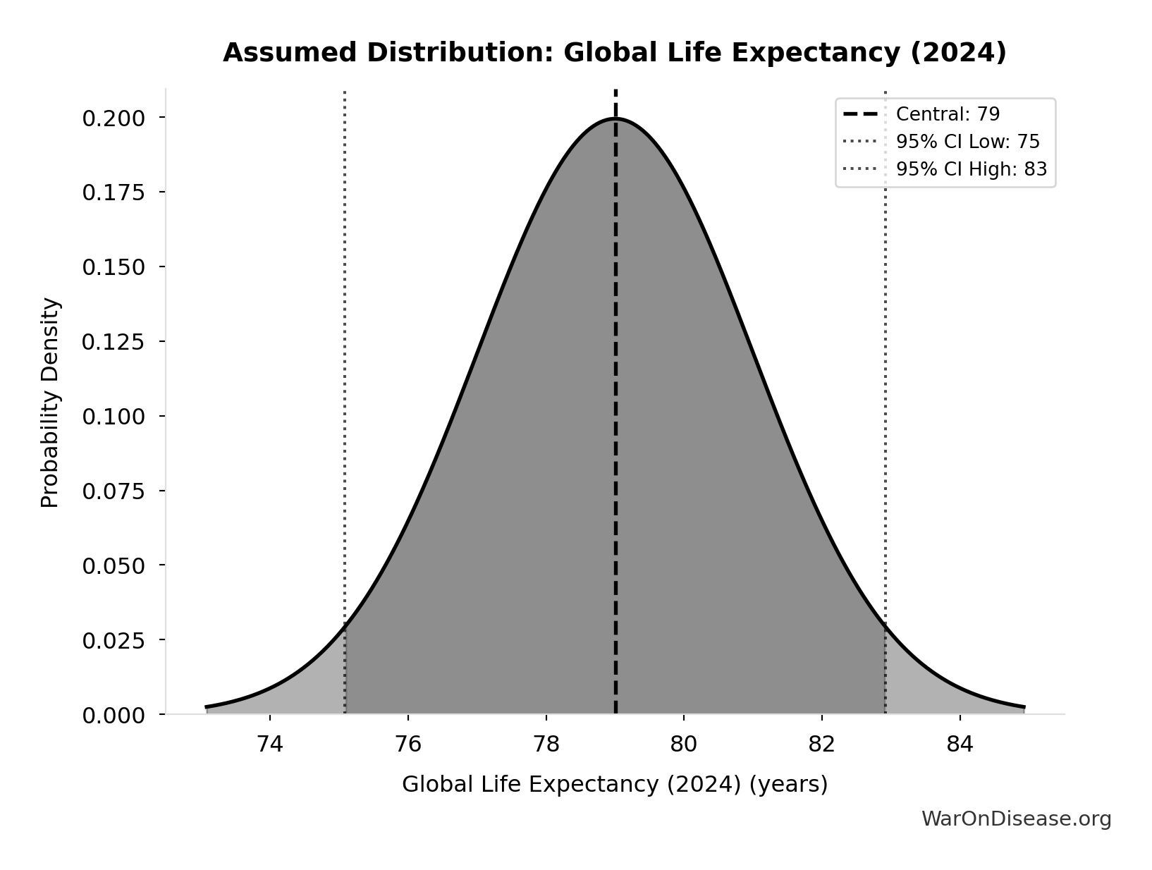
Global Life Expectancy (2024): 79 years
Global life expectancy (2024)
Source:18
Uncertainty Range
Technical: Distribution: Normal (SE: 2 years)
Input Distribution
This chart shows the assumed probability distribution for this parameter. The shaded region represents the 95% confidence interval where we expect the true value to fall.
✓ High confidence • 📊 Peer-reviewed • Updated 2024
Pharma Drug Development Cost (Current System): $2.60B
Average cost to develop one drug in current system
Source:82
Uncertainty Range
Technical: 95% CI: [$1.50B, $4B] • Distribution: Lognormal (SE: $500M)
What this means: There’s significant uncertainty here. The true value likely falls between $1.50B and $4B (±48%). This represents a wide range that our Monte Carlo simulations account for when calculating overall uncertainty in the results.
The lognormal distribution means values can’t go negative and have a longer tail toward higher values (common for costs and populations).
Input Distribution
This chart shows the assumed probability distribution for this parameter. The shaded region represents the 95% confidence interval where we expect the true value to fall.
✓ High confidence • 📊 Peer-reviewed
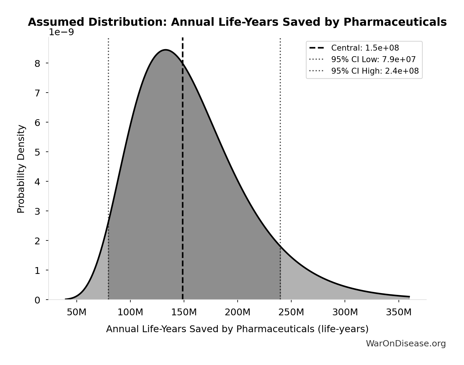
Annual Life-Years Saved by Pharmaceuticals: 149M life-years
Annual life-years saved by pharmaceutical innovations globally. Lichtenberg (2019, NBER WP 25483) found that drugs launched after 1981 saved 148.7M life-years in 2013 across 22 countries using 3-way fixed-effects regression (disease-country-year). 95% CI [79.4M, 239.8M] propagated from Table 2 regression standard errors (β₀₋₁₁=-0.031±0.008, β₁₂₊=-0.057±0.013).
Source:84
Uncertainty Range
Technical: 95% CI: [79.4M life-years, 240M life-years] • Distribution: Lognormal
What this means: This estimate is highly uncertain. The true value likely falls between 79.4M life-years and 240M life-years (±54%). This represents a very wide range that our Monte Carlo simulations account for when calculating overall uncertainty in the results.
The lognormal distribution means values can’t go negative and have a longer tail toward higher values (common for costs and populations).
Input Distribution
This chart shows the assumed probability distribution for this parameter. The shaded region represents the 95% confidence interval where we expect the true value to fall.
~ Medium confidence
Pharma Drug Success Rate (Current System): 10%
Percentage of drugs that reach market in current system
Source:86
✓ High confidence • 📊 Peer-reviewed
Phase I Safety Trial Duration: 2.3 years
Post-1962 Drug Approval Reduction: 70%
Reduction in new drug approvals after 1962 Kefauver-Harris Amendment (70% drop from 43→17 drugs/year)
Source:95
✓ High confidence • Updated 1962-1970
Pre-1962 Physician Count (Unverified): 144k physicians
Estimated physicians conducting real-world efficacy trials pre-1962 (unverified estimate)
Source:98
? Low confidence
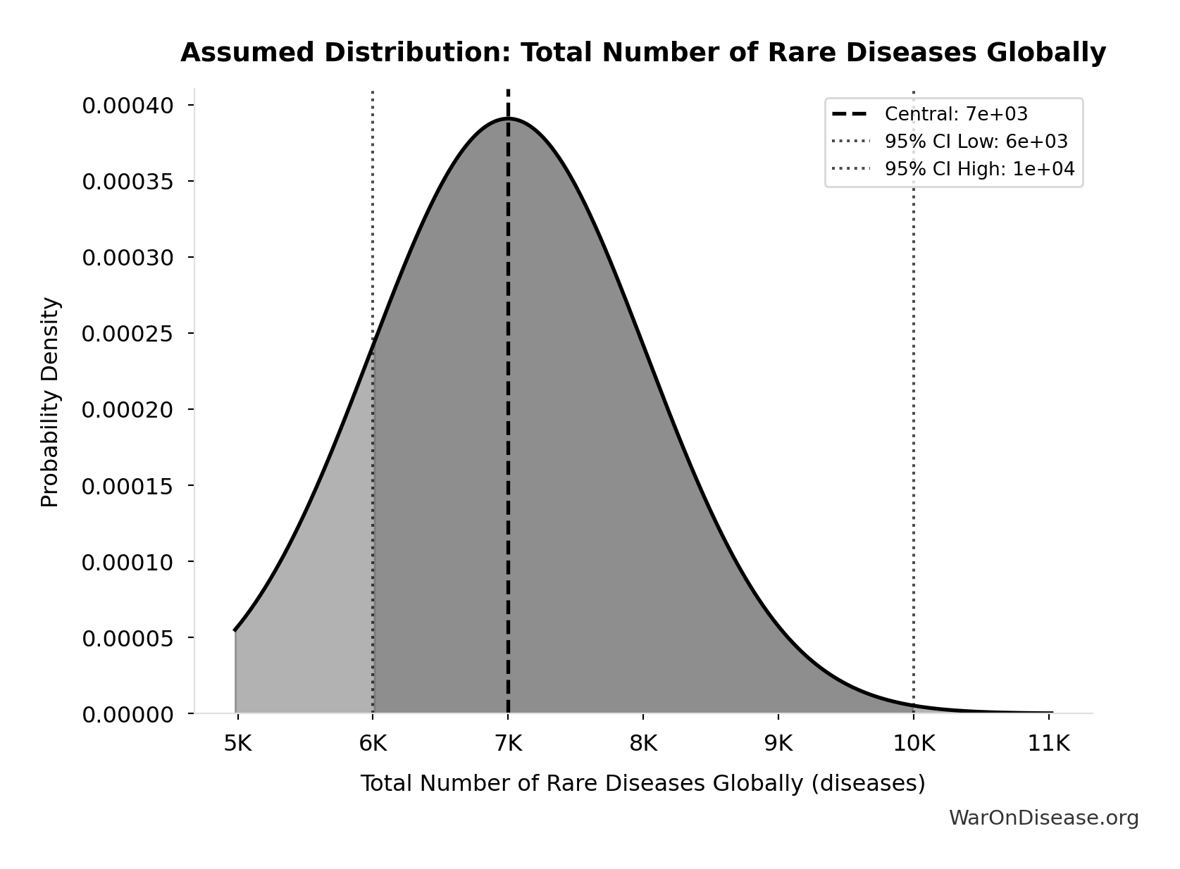
Total Number of Rare Diseases Globally: 7.00k diseases
Total number of rare diseases globally
Source:99
Uncertainty Range
Technical: 95% CI: [6.00k diseases, 10.0k diseases] • Distribution: Normal
What this means: There’s significant uncertainty here. The true value likely falls between 6.00k diseases and 10.0k diseases (±29%). This represents a wide range that our Monte Carlo simulations account for when calculating overall uncertainty in the results.
The normal distribution means values cluster around the center with equal chances of being higher or lower.
Input Distribution
This chart shows the assumed probability distribution for this parameter. The shaded region represents the 95% confidence interval where we expect the true value to fall.
✓ High confidence
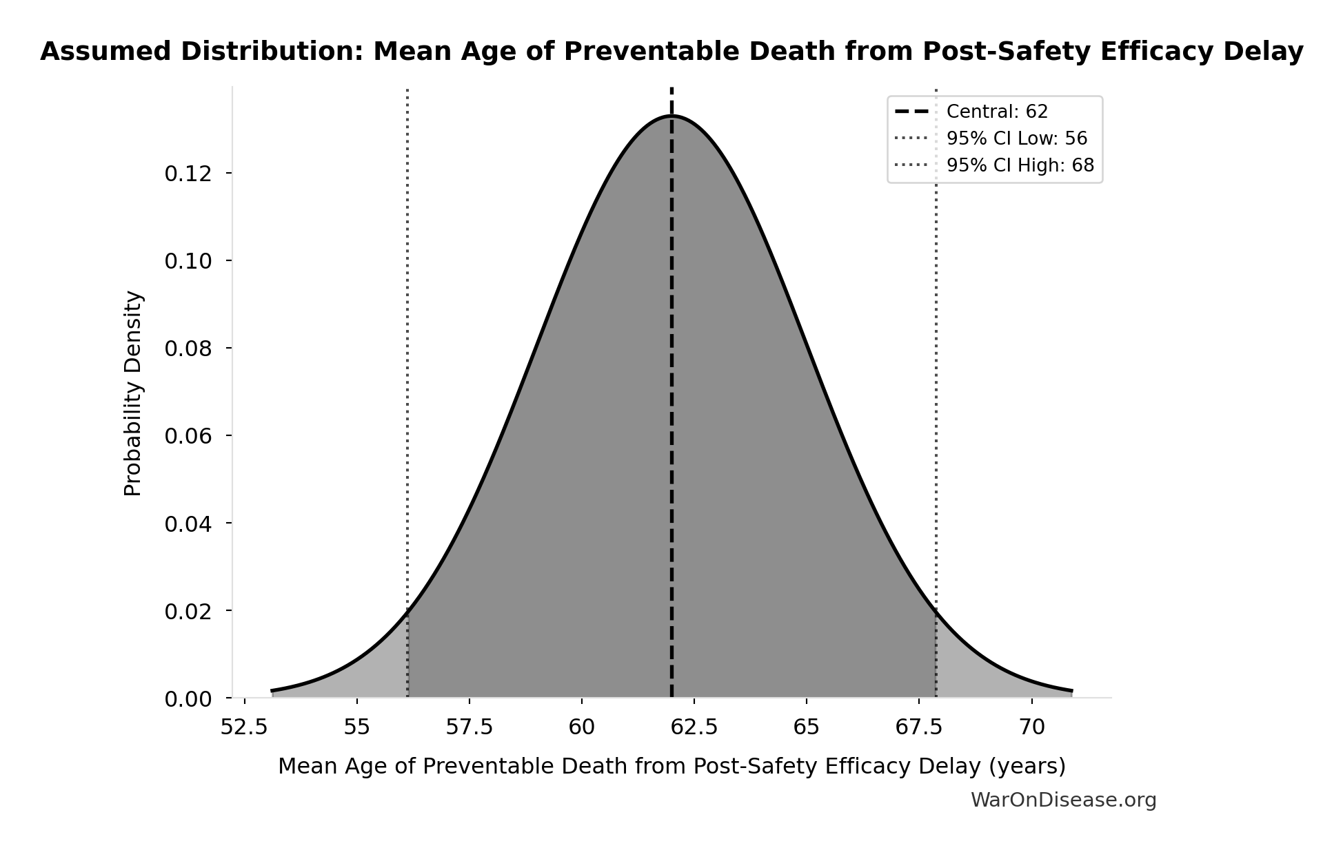
Mean Age of Preventable Death from Post-Safety Efficacy Delay: 62 years
Mean age of preventable death from post-safety efficacy testing regulatory delay (Phase 2-4)
Source:18
Uncertainty Range
Technical: Distribution: Normal (SE: 3 years)
Input Distribution
This chart shows the assumed probability distribution for this parameter. The shaded region represents the 95% confidence interval where we expect the true value to fall.
~ Medium confidence • 📊 Peer-reviewed
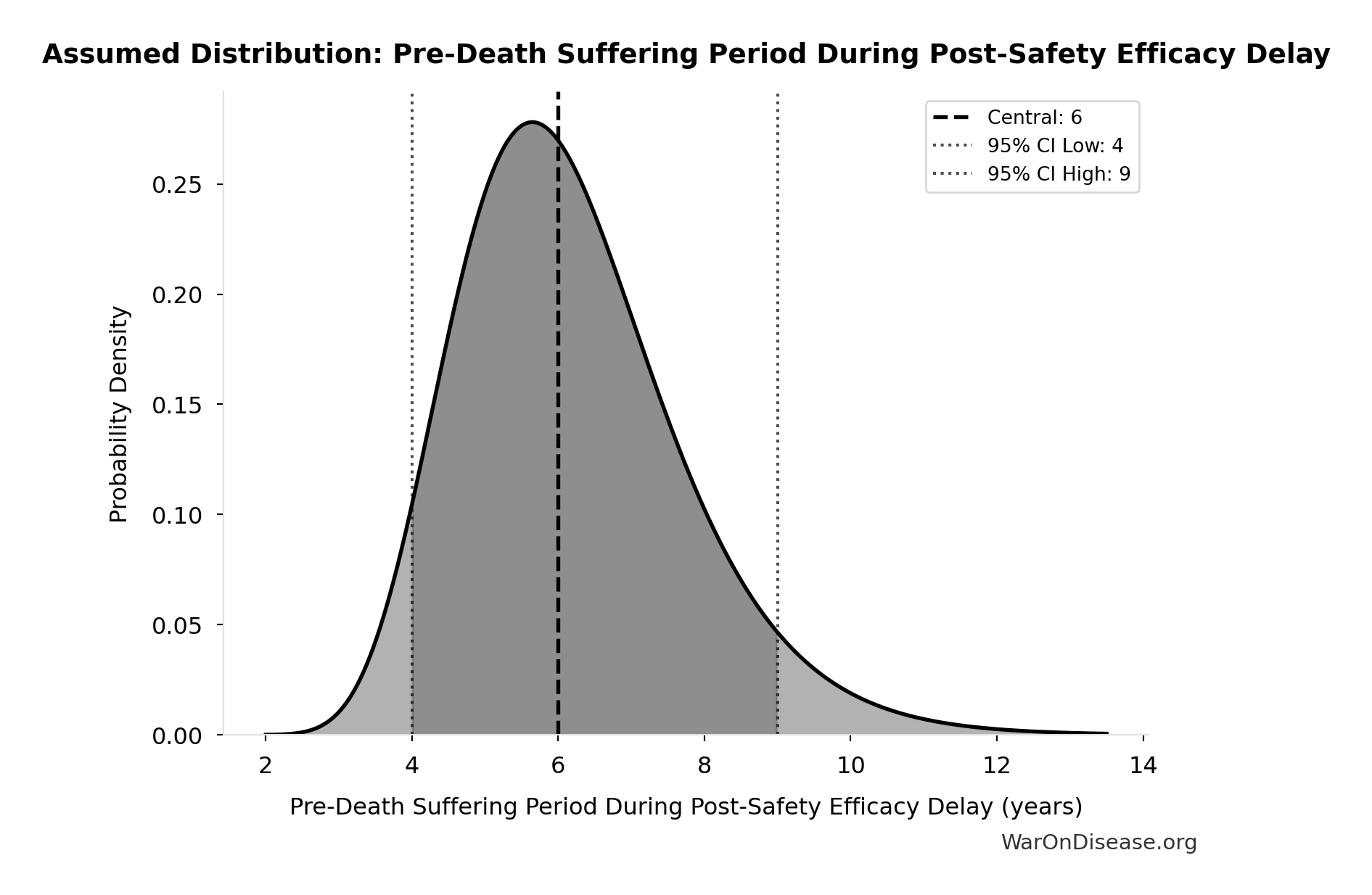
Pre-Death Suffering Period During Post-Safety Efficacy Delay: 6 years
Pre-death suffering period during post-safety efficacy testing delay (average years lived with untreated condition while awaiting Phase 2-4 completion)
Source:18
Uncertainty Range
Technical: 95% CI: [4 years, 9 years] • Distribution: Lognormal
What this means: There’s significant uncertainty here. The true value likely falls between 4 years and 9 years (±42%). This represents a wide range that our Monte Carlo simulations account for when calculating overall uncertainty in the results.
The lognormal distribution means values can’t go negative and have a longer tail toward higher values (common for costs and populations).
Input Distribution
This chart shows the assumed probability distribution for this parameter. The shaded region represents the 95% confidence interval where we expect the true value to fall.
~ Medium confidence • 📊 Peer-reviewed
September 11 Deaths: 2.98k people
Total deaths in the September 11, 2001 attacks. 2,977 victims (excluding 19 hijackers). Used as a reference point for scale comparisons.
Source:102
Uncertainty Range
Technical: Distribution: Fixed
✓ High confidence
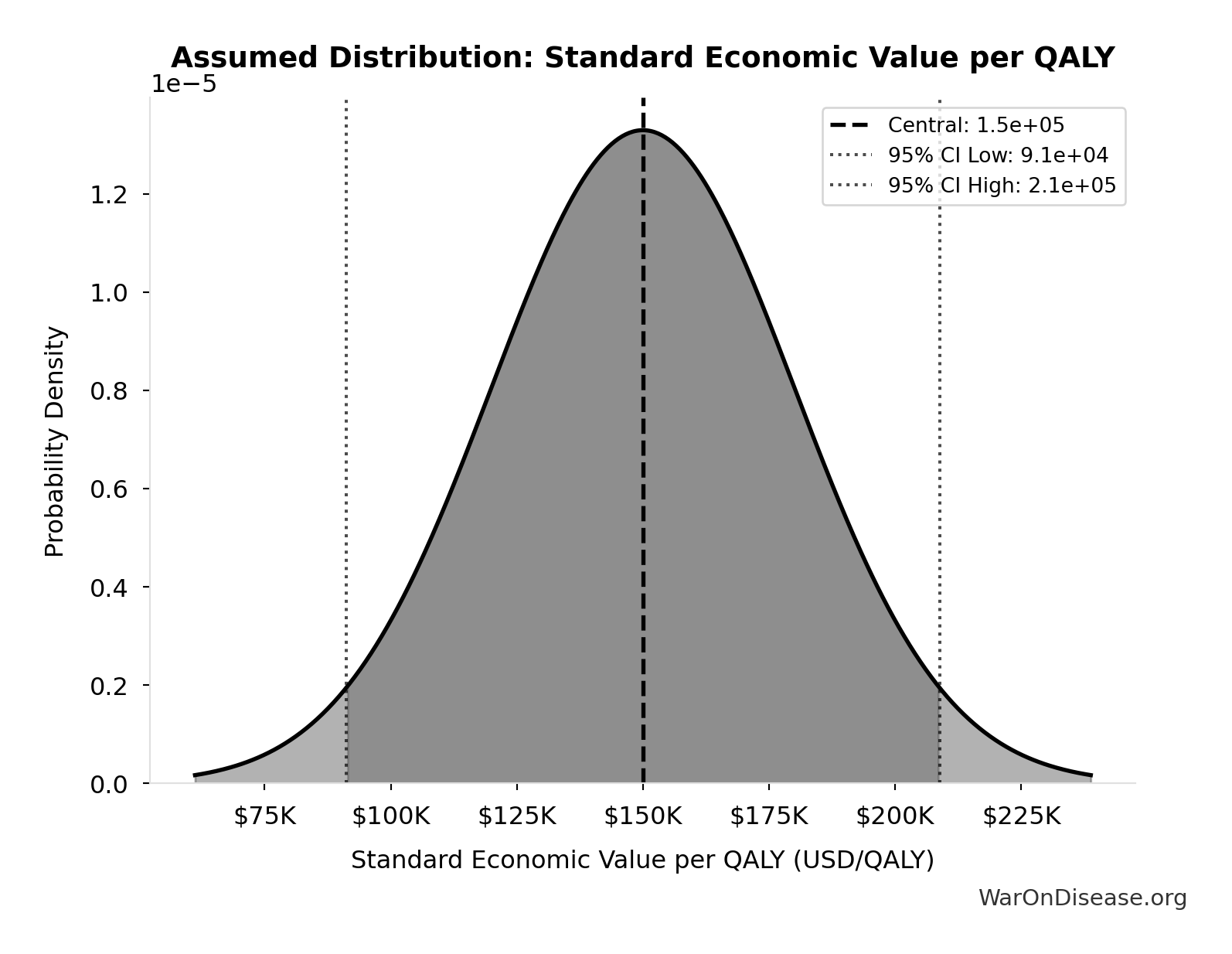
Standard Economic Value per QALY: $150K
Standard economic value per QALY
Source:108
Uncertainty Range
Technical: Distribution: Normal (SE: $30K)
Input Distribution
This chart shows the assumed probability distribution for this parameter. The shaded region represents the 95% confidence interval where we expect the true value to fall.
✓ High confidence
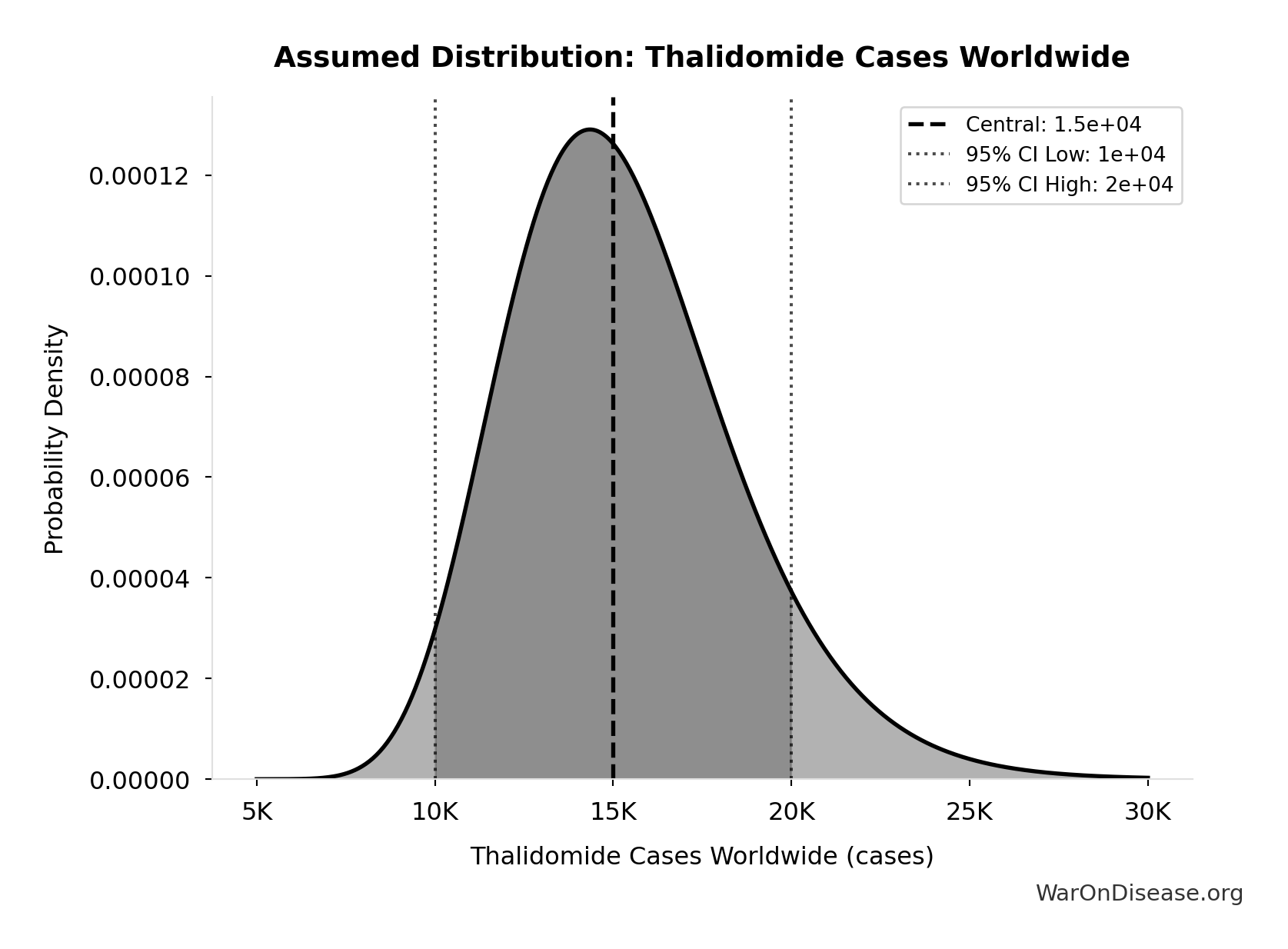
Thalidomide Cases Worldwide: 15.0k cases
Total thalidomide birth defect cases worldwide (1957-1962)
Source:115
Uncertainty Range
Technical: 95% CI: [10.0k cases, 20.0k cases] • Distribution: Lognormal
What this means: There’s significant uncertainty here. The true value likely falls between 10.0k cases and 20.0k cases (±33%). This represents a wide range that our Monte Carlo simulations account for when calculating overall uncertainty in the results.
The lognormal distribution means values can’t go negative and have a longer tail toward higher values (common for costs and populations).
Input Distribution
This chart shows the assumed probability distribution for this parameter. The shaded region represents the 95% confidence interval where we expect the true value to fall.
~ Medium confidence
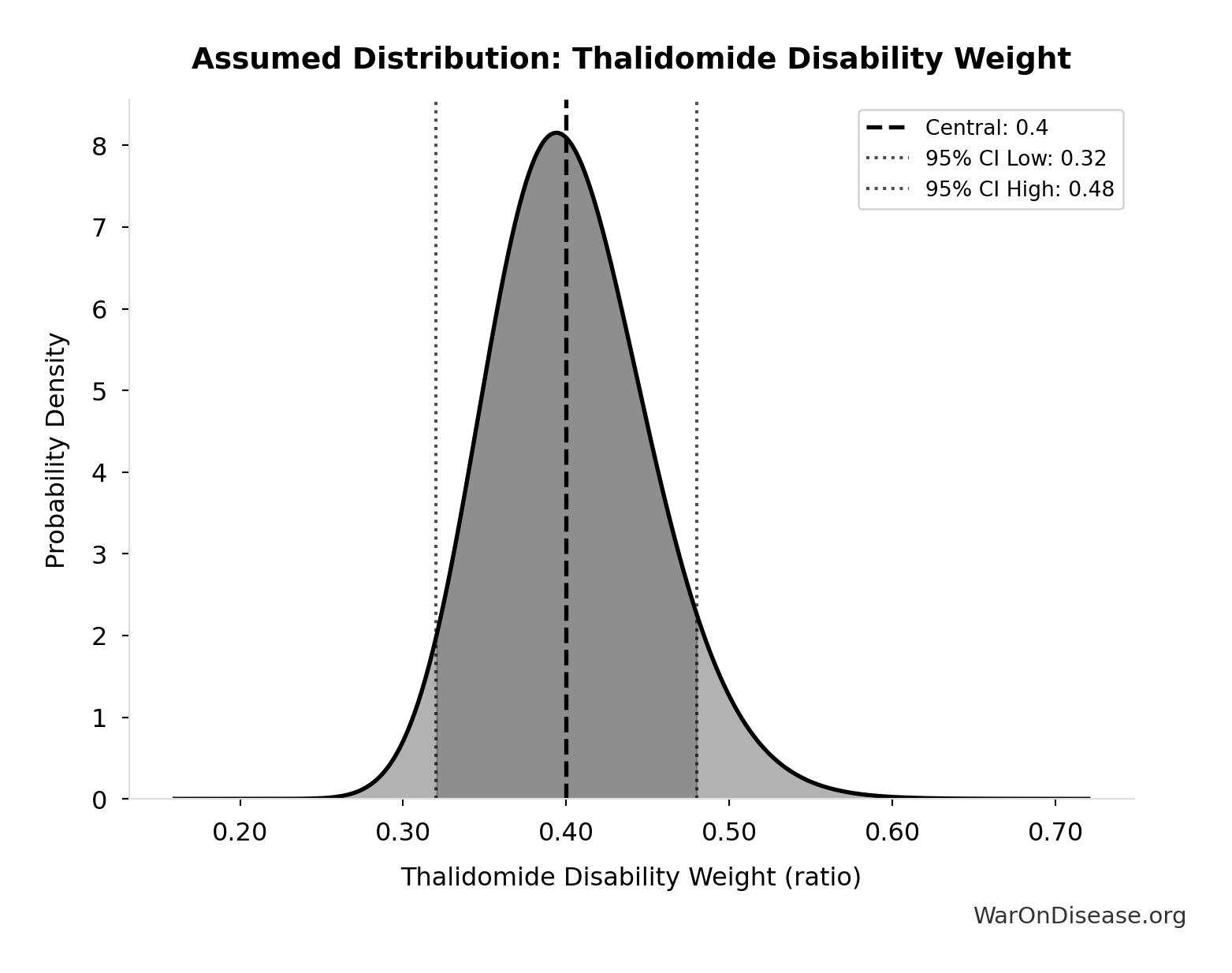
Thalidomide Disability Weight: 0.4:1
Disability weight for thalidomide survivors (limb deformities, organ damage)
Source:116
Uncertainty Range
Technical: 95% CI: [0.32:1, 0.48:1] • Distribution: Lognormal
What this means: This estimate has moderate uncertainty. The true value likely falls between 0.32:1 and 0.48:1 (±20%). This represents a reasonable range that our Monte Carlo simulations account for when calculating overall uncertainty in the results.
The lognormal distribution means values can’t go negative and have a longer tail toward higher values (common for costs and populations).
Input Distribution
This chart shows the assumed probability distribution for this parameter. The shaded region represents the 95% confidence interval where we expect the true value to fall.
~ Medium confidence
Thalidomide Mortality Rate: 40%
Mortality rate for thalidomide-affected infants (died within first year)
Source:115
Uncertainty Range
Technical: 95% CI: [35%, 45%] • Distribution: Lognormal
What this means: This estimate has moderate uncertainty. The true value likely falls between 35% and 45% (±13%). This represents a reasonable range that our Monte Carlo simulations account for when calculating overall uncertainty in the results.
The lognormal distribution means values can’t go negative and have a longer tail toward higher values (common for costs and populations).
Input Distribution
This chart shows the assumed probability distribution for this parameter. The shaded region represents the 95% confidence interval where we expect the true value to fall.
✓ High confidence
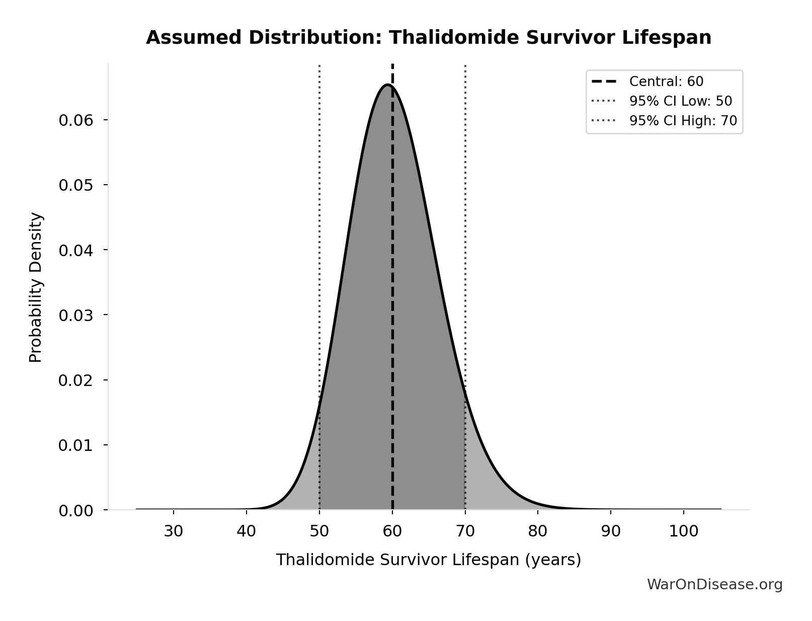
Thalidomide Survivor Lifespan: 60 years
Average lifespan for thalidomide survivors
Source:116
Uncertainty Range
Technical: 95% CI: [50 years, 70 years] • Distribution: Lognormal
What this means: This estimate has moderate uncertainty. The true value likely falls between 50 years and 70 years (±17%). This represents a reasonable range that our Monte Carlo simulations account for when calculating overall uncertainty in the results.
The lognormal distribution means values can’t go negative and have a longer tail toward higher values (common for costs and populations).
Input Distribution
This chart shows the assumed probability distribution for this parameter. The shaded region represents the 95% confidence interval where we expect the true value to fall.
~ Medium confidence
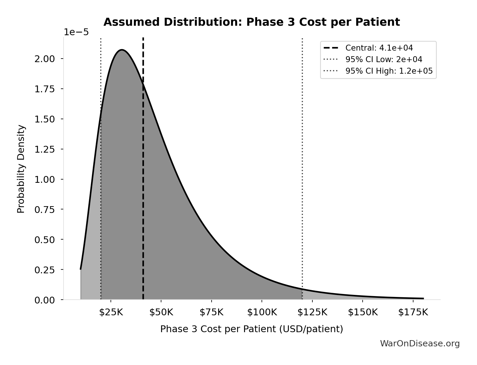
Phase 3 Cost per Patient: $41K
Phase 3 cost per patient (median from FDA study)
Source:118
Uncertainty Range
Technical: 95% CI: [$20K, $120K] • Distribution: Lognormal
What this means: This estimate is highly uncertain. The true value likely falls between $20K and $120K (±122%). This represents a very wide range that our Monte Carlo simulations account for when calculating overall uncertainty in the results.
The lognormal distribution means values can’t go negative and have a longer tail toward higher values (common for costs and populations).
Input Distribution
This chart shows the assumed probability distribution for this parameter. The shaded region represents the 95% confidence interval where we expect the true value to fall.
✓ High confidence
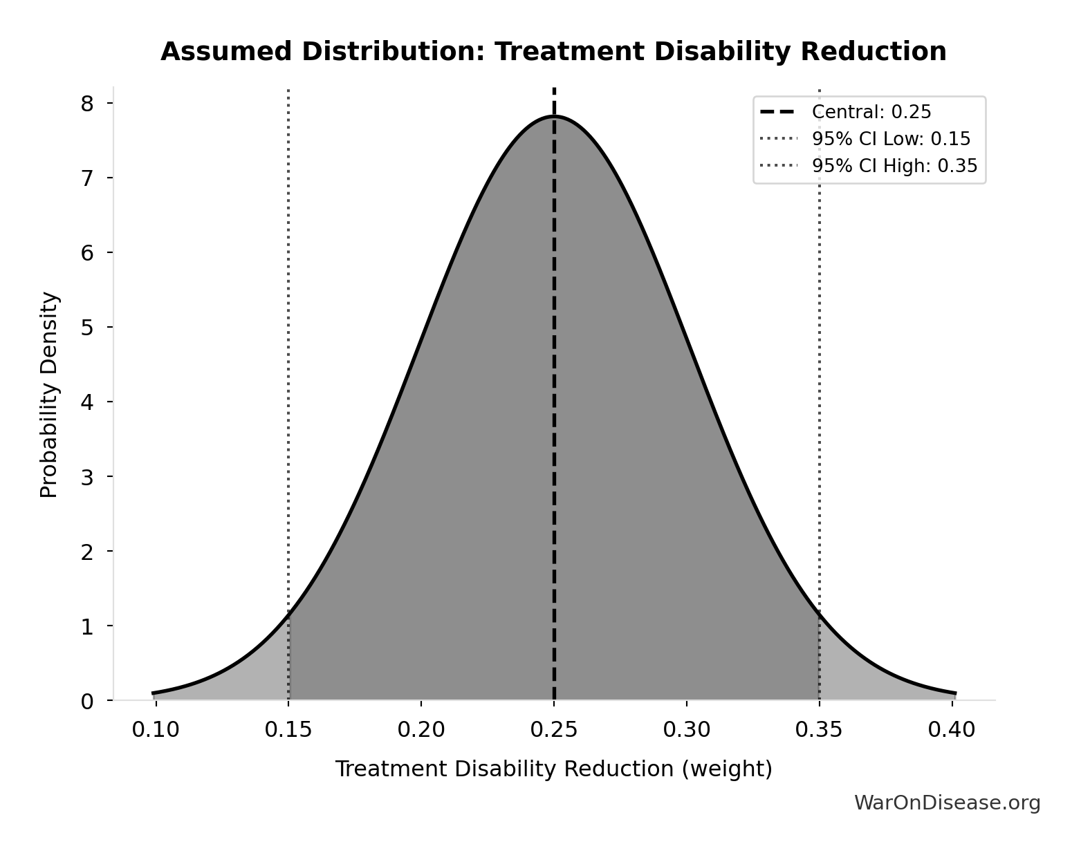
Treatment Disability Reduction: 0.25 weight
Average disability weight reduction from pharmaceutical treatment. Untreated chronic disease averages 0.35 disability weight, treated disease averages 0.10, difference is 0.25.
Source:119
Uncertainty Range
Technical: 95% CI: [0.15 weight, 0.35 weight] • Distribution: Normal
What this means: There’s significant uncertainty here. The true value likely falls between 0.15 weight and 0.35 weight (±40%). This represents a wide range that our Monte Carlo simulations account for when calculating overall uncertainty in the results.
The normal distribution means values cluster around the center with equal chances of being higher or lower.
Input Distribution
This chart shows the assumed probability distribution for this parameter. The shaded region represents the 95% confidence interval where we expect the true value to fall.
~ Medium confidence • 📊 Peer-reviewed
Core Definitions
Fundamental parameters and constants used throughout the analysis.
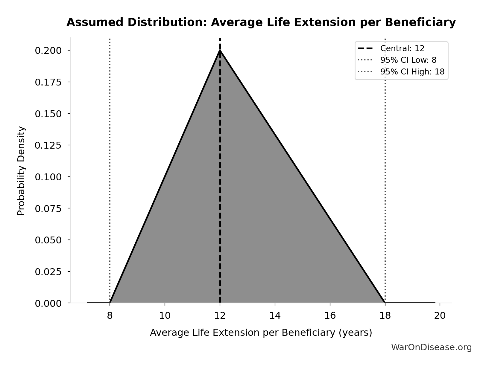
Average Life Extension per Beneficiary: 12 years
Average years of life extension per person saved by pharmaceutical interventions. Assumption used to convert life-years saved to approximate lives saved. Based on Lichtenberg’s methodology where life-years are calculated from Years of Life Lost (YLL) reductions.
Uncertainty Range
Technical: 95% CI: [8 years, 18 years] • Distribution: Triangular
What this means: There’s significant uncertainty here. The true value likely falls between 8 years and 18 years (±42%). This represents a wide range that our Monte Carlo simulations account for when calculating overall uncertainty in the results.
The triangular distribution means values cluster around a most-likely point but can range higher or lower.
Input Distribution
This chart shows the assumed probability distribution for this parameter. The shaded region represents the 95% confidence interval where we expect the true value to fall.
Core definition
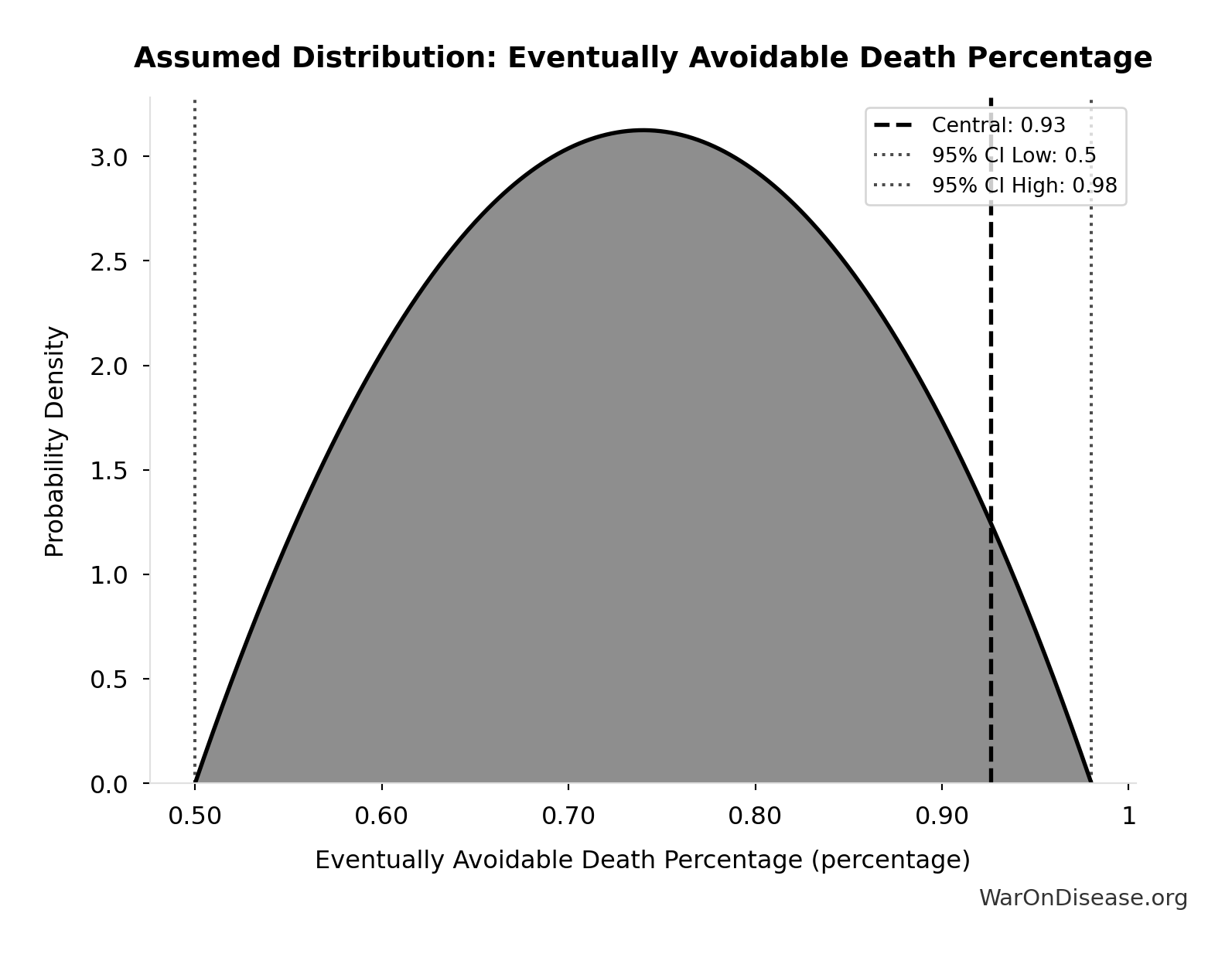
Eventually Avoidable Death Percentage: 92.6%
Percentage of deaths that are eventually avoidable with sufficient biomedical research and technological advancement. Central estimate ~92% based on ~7.9% fundamentally unavoidable (primarily accidents). Wide uncertainty reflects debate over: (1) aging as addressable vs. fundamental, (2) asymptotic difficulty of last diseases, (3) multifactorial disease complexity.
Uncertainty Range
Technical: 95% CI: [50%, 98%] • Distribution: Beta
What this means: There’s significant uncertainty here. The true value likely falls between 50% and 98% (±26%). This represents a wide range that our Monte Carlo simulations account for when calculating overall uncertainty in the results.
The beta distribution means values are bounded and can skew toward one end.
Input Distribution
This chart shows the assumed probability distribution for this parameter. The shaded region represents the 95% confidence interval where we expect the true value to fall.
Core definition
Standard Discount Rate for NPV Analysis: 3%
Standard discount rate for NPV analysis (3% annual, social discount rate)
Uncertainty Range
Technical: Distribution: Fixed
Core definition
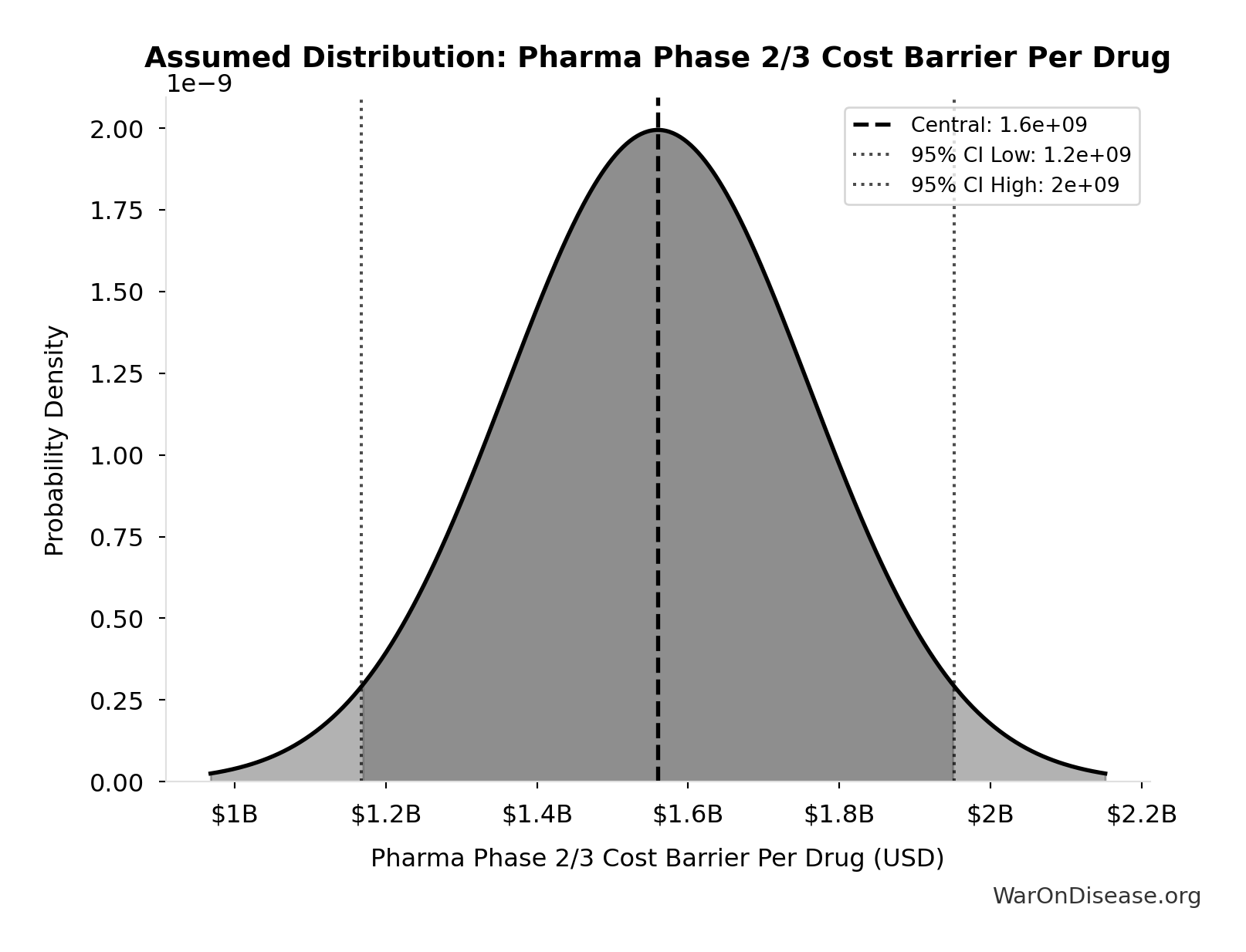
Pharma Phase 2/3 Cost Barrier Per Drug: $1.56B
Average Phase 2/3 efficacy testing cost per drug that pharma must fund (~60% of $2.6B total)
Uncertainty Range
Technical: Distribution: Normal (SE: $200M)
Input Distribution
This chart shows the assumed probability distribution for this parameter. The shaded region represents the 95% confidence interval where we expect the true value to fall.
Core definition
